Taming Polysemanticity in LLMs: Provable Feature Recovery via Sparse Autoencoders

Abstract

We address the challenge of theoretically grounded feature recovery using Sparse Autoencoders (SAEs) for interpreting Large Language Models. Current SAE training methods lack mathematical guarantees and face issues like hyperparameter sensitivity. We propose a statistical framework for feature recovery that models polysemantic features as sparse mixtures of monosemantic concepts. Based on this, we develop a "bias adaptation" SAE training algorithm that dynamically adjusts network biases for optimal sparsity. We prove that this algorithm correctly recovers all monosemantic features under our statistical model. Our improved variant, Group Bias Adaptation (GBA), outperforms existing methods on LLMs up to 1.5 billion parameters in terms of sparsity-loss trade-off and feature consistency. This work provides the first SAE algorithm with theoretical recovery guarantees, advancing interpretable and trustworthy AI through enhanced mechanistic understanding.

Key Contributions

A novel statistical framework that rigorously formalizes feature recovery by modeling polysemantic features as sparse combinations of underlying monosemantic concepts, and establishes a precise notion of feature identifiability.

An innovative SAE training algorithm, Group Bias Adaptation (GBA), which adaptively adjusts neural network bias parameters to enforce optimal activation sparsity, allowing distinct groups of neurons to target different activation frequencies.

The first theoretical guarantee proving that SAE training algorithm can provably recover all monosemantic features when the input data is sampled from our proposed statistical model.

Superior empirical performance on LLMs up to 1.5B parameters, where GBA achieves the best sparsity-loss trade-off while learning more consistent features than benchmark methods.

Introduction

BACKGROUND 1: FEATURE RECOVERY

To understand the task of feature recovery, let us consider the following example sentence:

The detective found a muddy footprint near the broken window, leading him to suspect a ?

The sentence contains two distinct concepts: a muddy footprint and a broken window. For a trained deep neural network, the learned representations in the intermediate layers are often polysemantic, meaning that they are mixture of multiple features of the underlying concepts. Specifically, the representation \(x\) after seeing the whole sentence may have the following form:

\(x = h_1 \cdot\) "feature of muddy footprint" \( + h_2 \cdot\) "feature of broken window"

where \(h_1\) and \(h_2\) are the nonnegative weights of the two monosemantic features. After obtaining the polysemantic representation \(x\), the model can then generate the token "burglary" at the "?" position.

The goal of feature recovery is to recover the monosemantic features underlying each concept, through training on a dataset that contains polysemantic representations, which are often extracted from the intermediate layers of a trained deep neural network, e.g., the residual stream of a transformer-based model.

While this example illustrates the intuitive notion of monosemantic features, we need a more rigorous definition to make progress. Currently, researchers primarily assess monosemanticity through feature interpretability, i.e., how well a feature aligns with human-understandable concepts. However, this anthropocentric view has limitations: neural networks may process information in ways fundamentally different from human conceptual understanding. We need a more principled, mathematically grounded definition of monosemantic features that captures their essential properties independent of human interpretation. Specifically, we ask the following questions:

Question 1

What is a mathematically rigorous definition of identifiable monosemantic features?

Question 2

Given polysemantic representations, when will the monosemantic features be identifiable?

Question 3

How to reliably recover the monosemantic features?

BACKGROUND 2: SPARSE AUTOENCODERS

📚 What are SAEs?

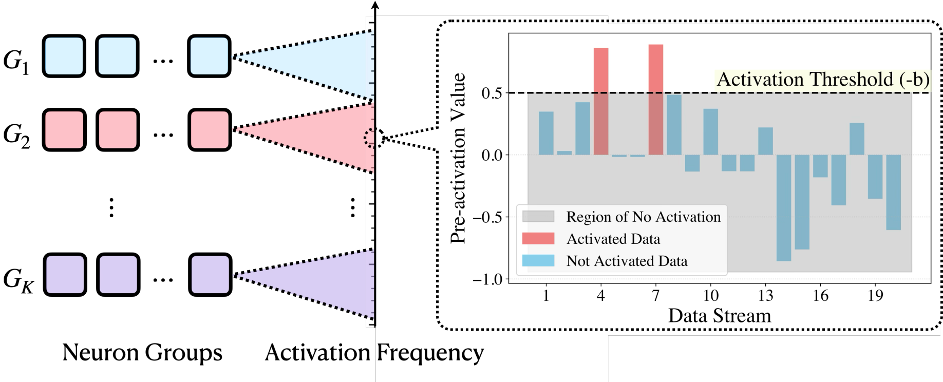
At the core of our feature recovery method is the Sparse Autoencoder (SAE), a neural network designed to learn sparse representations through self-reconstruction. A typical SAE architecture (with weight sharing between encoding and decoding layers) can be described as follows: \[ \hat x = \sum_{m=1}^M a_{m} \cdot w_{m} \cdot \phi\bigl( \underbrace{{w_{m}^\top (x-b_{\mathrm{pre}}) + b_{m}}}_{\displaystyle \small\text{pre-activation}~y_m} \bigr) + b_{\mathrm{pre}}, \] where each \(m\) index a neuron in the SAE, \(w_m\in \mathbb{R}^d\) is the tied weight vector for both encoding and decoding, \(a_m\in \mathbb{R}\) is the output scale for neuron \(m\), \(b_m\in \mathbb{R}\) is the bias for neuron \(m\), and \(b_{\mathrm{pre}}\in \mathbb{R}^d\) is the pre-bias vector that centers the input data. People usually use some nonlinear activation function \(\phi\) like ReLU or JumpReLU.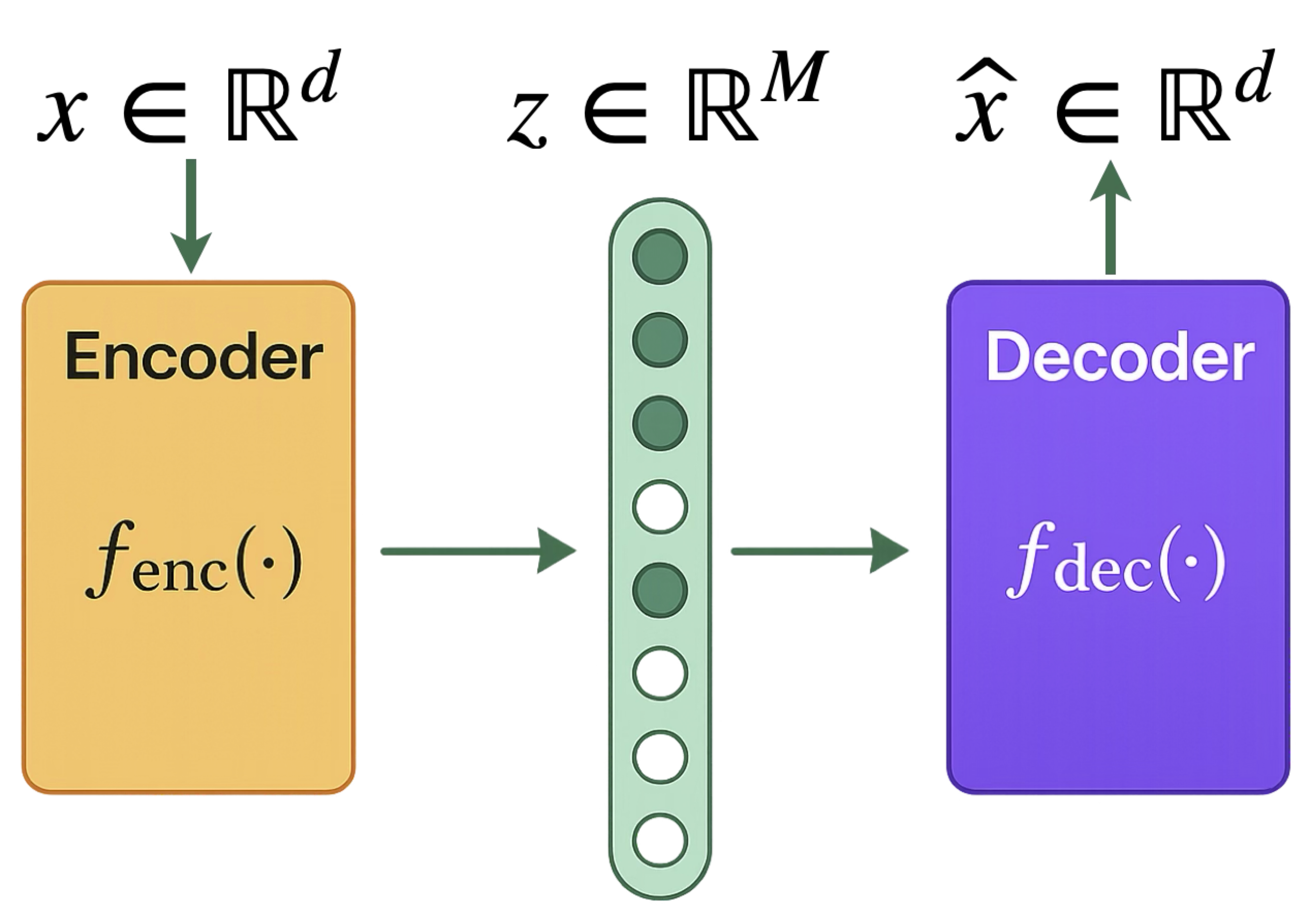

Illustration of neuron grouping and bias adaptation — Figure 1: Sparse Autoencoder Architecture, where the latent representation \(z\in\mathbb{R}^M\) is obtained by passing the pre-activation \(y_m\) through the activation function \(\phi\).

🔧 How are SAEs trained?

Given the input \(x\in \mathbb{R}^d\), the SAE outputs \(\hat x\in \mathbb{R}^d\) as the reconstruction, and the training objective is to minimize the reconstruction error with a regularization term to encourage sparsity. Specifically, the training objective for the \(\ell_1\) method is to minimize the following loss function: \[ \mathcal{L} = \mathbb{E}_{x\sim \mathcal{D}} \biggl[\underbrace{ (\hat x - x)^2}_{\displaystyle \small\text{reconstruction loss}} + \underbrace{\lambda \sum_{m=1}^M \|w_m\|_2 \phi(w_m^\top (x - b_{\mathrm{pre}}) + b_m)}_{\displaystyle \small\text{sparsity regularization}} \biggr]. \] where \(\mathcal{D}\) is the training dataset, and \(\lambda\) is the regularization parameter. The first term is the reconstruction loss, and the second term is the sparsity regularization term. The sparsity regularization term encourages the SAE to activate only a small number of neurons, which is crucial for feature recovery. The TopK method does not have a regularization term, and the activation frequency is controlled by only allowing the top-K neurons in terms of the pre-activation \(y_m\) to be activated.

🤔 Why using SAEs?

The hypothesis is that by enforcing activation sparsity, SAEs can decompose polysemantic representations (a mixture of multiple features) into monosemantic features (which each correspond to a single interpretable concept). Empirically, SAEs have been shown to learn interpretable features for LLMs.

WHAT ARE THE CHALLENGES

The current SAE training algorithms face the following challenges:

Theoretical uncertainty: We lack clear feature definitions and current SAE training algorithms lack theoretical guarantees, making reliable feature recovery uncertain.
Hyperparameter sensitivity: Empirically, \( \ell_1 \) regularization and TopK activation methods are sensitive to hyperparameters tuning.
Feature inconsistency: TopK activation methods produce inconsistent features across different random seeds.¹

WHAT ARE OUR GOALS

Our research aims to address these challenges with the following objectives:

Theoretical foundation: Develop a rigorous mathematical framework for understanding and analyzing feature recovery in SAEs.
Algorithm design: Create a simple and robust training algorithm that can reliably recover monosemantic features without extensive hyperparameter tuning, and learn more consistent features across different random seeds.

Ultimately, our research aims to establish a rigorous foundation for mechanistic interpretability research, bringing us closer to realizing our interpretability dreams² of understanding the inner workings of neural networks.

¹Paulo, Gonçalo, and Nora Belrose. "Sparse Autoencoders Trained on the Same Data Learn Different Features." https://arxiv.org/abs/2501.16615
²Chris Olah. "Interpretability Dreams." https://transformer-circuits.pub/2023/interpretability-dreams/index.html

Algorithm Design

To address the limitations of existing Sparse Autoencoder (SAE) training methods, we propose a new algorithm called Grouped Bias Adaptation (GBA). Our algorithm has two main components: a bias adaptation subroutine that controls the activation frequency of each neuron, and a neuron grouping strategy that allows us to assign different target activation frequencies (TAFs) to different groups of neurons. The algorithm is carried out as follows:

👥 Before the training: Neuron Grouping with TAFs

We divide the neurons into some groups (let us denote each group as \(G_k\), and the group index as \(k=1,2,\ldots,K\)), and each group has a unique TAF \(p_k\).
During the training, we wish the activation frequency (fraction of data on which the neuron is activated) for neurons within each group to be close to \(p_k\).
We typically use a geometric sequence starting at a high frequency, e.g., 0.1, and decreasing to a low frequency, e.g., 0.001, for assigning the TAFs to capture both the common and rare features.

🔄 During the training: Bias Adaptation to Achieve TAFs
During training, we perform two main operations:

Minimize reconstruction loss by performing gradient steps on the weights \((w_m, a_m, b_{\mathrm{pre}})\) except for the biases.
Dynamically adjust neuron biases based on activation frequency in a data buffer:
- If a neuron activates more frequently than its TAF → decrease its bias to reduce activation
- If a neuron activates less frequently than its TAF → increase its bias to encourage activation

This dual approach maintains balanced neuron activation and prevents "dead" neurons.

By combining these two strategies, GBA offers direct control over neuron activation, avoiding the need for complex tuning while ensuring that neurons are activated at appropriate frequencies to learn features that also occur with different frequencies.

SAE Training on Qwen2.5-1.5B

In this section, we evaluate the performance of our Grouped Bias Adaptation (GBA) algorithm across several key dimensions. To ensure a comprehensive understanding, we first briefly introduce the experimental setup before diving into the analysis of the three key questions.

Experimental Setup

We conduct our experiments using two datasets: Pile Github and Pile Wikipedia datasets, each with the first 100k tokens. The experiments are performed on the Qwen2.5-1.5B base model, where we attach a Sparse Autoencoder (SAE) to the MLP outputs of layers 2, 13, and 26. Each SAE contains 66k hidden neurons and operates with an input/output dimension of 1536. To ensure optimal performance, we adopt the JumpReLU activation function for all methods tested. We use 100 million tokens for training the SAEs, feeding the tokens through the LLM and collecting the MLP outputs at the specified layers. The four methods compared are:

TopK: A sparse activation method that retains only the top-K activated neurons.
L1: A sparse method that uses L1 regularization for sparsity.
BA (Bias Adaptation): A variant of GBA with a single group and hyperparameter tuning for Target Activation Frequency (TAF).
GBA (Grouped Bias Adaptation): Our proposed method, which uses multiple groups of neurons with TAFs set geometrically without hyperparameter tuning.

All methods were trained using the AdamW optimizer with the same set of hyperparameters, including learning rate, weight decay, and batch size. In the GBA method, we used 10 groups, with the Highest Target Frequency (HTF) set to 0.1 and the Lowest Target Frequency (LTF) set to 0.001.

Reconstruction Loss and Activation Sparsity Frontier

The first question we address is how the GBA method compares with other methods in terms of reconstruction loss and activation sparsity. The results show that GBA performs comparably to the TopK method with post-activation sparsity and outperforms it with pre-activation sparsity. Furthermore, GBA significantly outperforms the L1 and Bias Adaptation (BA) methods across all experiments.

🎯Finding (1): GBA performs comparably to the best-performing benchmark, TopK with post-activation sparsity. In addition, GBA outperforms TopK with pre-activation sparsity. Specifically, when these methods have the same average fraction of activated neurons, GBA's reconstruction is comparable to that of TopK with post-activation sparsity and significantly better than that of TopK with pre-activation sparsity.
🏆Finding (2): GBA outperforms L1 significantly. When they have the same average fraction of activated neurons, GBA achieves a lower reconstruction loss.
🏆Finding (3): GBA outperforms BA consistently across all experiments. This provides strong evidence that the grouping mechanism enhances both sparsity and reconstruction performance.

Reconstruction loss vs activation sparsity — Figure 3: Reconstruction loss versus the average fraction of activated neurons for various methods. The GBA method shows competitive performance with the TopK method.

Robustness and Nearly Tuning-Free

The second question revolves around the robustness of the GBA method to the choice of hyperparameters, such as the number of groups and target frequencies. Our ablation studies show that GBA is nearly tuning-free. As long as the Highest Target Frequency (HTF) is sufficiently high (e.g., 0.5) and the number of groups (K) is large enough (e.g., 10 or 20), GBA performs consistently well.

🎯Finding (4): When HTF and LTF are properly chosen (e.g., a high HTF and a modestly low LTF), with an adequate number of groups, the GBA method achieves performance comparable to TopK, and the performance becomes largely insensitive to the specific choices of these parameters.

Ablation study on GBA robustness — Figure 4: Ablation study showing the robustness of GBA to different choices of the Highest Target Frequency (HTF) and the number of groups (K).

Consistency of Recovered Features

The third question examines the consistency of the features learned by the GBA method across independent runs with different random seeds. We evaluate this using the Maximum Cosine Similarity (MCS) metric, and the results show that GBA outperforms other methods, including TopK, in terms of feature consistency. The specific definition of MCS can be found in §A.2 (Evaluation Metrics) of the paper. Simply put, a higher MCS indicates that a neuron can find another neuron that is more similar to it in other runs, with higher values indicating better consistency. Speicifically, we plot the percentage of neurons that has MCS higher than different thresholds, where the neurons ploted are also filtered by certain metrics.

🏆Finding (5): As the TopK method is shown to be seed-dependent, it has the lowest MCS overall. Our GBA method outperforms TopK in achieving a higher percentage of neurons with high MCS.
🎯Finding (6): The L1 method is more consistent than TopK uniformly and more consistent than GBA in three of the four cases. However, when focusing on neurons with the top-0.05% activations, our GBA method surpasses the L1 method.

Consistency of features across runs — Figure 5: Consistency of recovered features measured by Maximum Cosine Similarity (MCS) across three runs with different random seeds. GBA outperforms other methods in feature consistency.

Additional Results

We provide additional studies on the neurons learned by the GBA in terms of the three metrics used above: maximum activation, Z-score, and maximum cosine similarity across different runs with different random seeds. These metrics are computed based on the validation part of the Pile Github dataset, with the hook position at the MLP output of layer 26. For each neuron, we also compute the activation fraction, which is the fraction of tokens where the pre-activations of the neuron are non-negative.

For each neuron, we have four metrics: maximum activation, Z-score, maximum cosine similarity, and activation fraction. We generate scatter plots by plotting the Z-score against the other three metrics. The results for GBA are shown below.

Scatter plots for neuron properties (GBA and TopK) — Figure 6: Scatter plots illustrating neuron properties for the GBA method: Z-score versus Maximum Activation, Fraction of Non-negative Pre-Activations (i.e., activation frequency), and Maximum Cosine Similarity across different runs with different random seeds. The 66k-neuron SAE is trained on the `Pile Github` dataset with a hook at the MLP output of layer 26.

Subplots Explanation

Left: Z-score vs Maximum Activation - This plot shows the relationship between the Z-score and maximum activation of neurons. We observe an almost linear relationship, indicating that neurons with higher Z-scores also have higher maximum activations.
Middle: Z-score vs Activation Fraction - This plot illustrates the correlation between the Z-score and the activation fraction. Neurons with higher Z-scores tend to have activation frequency close to 0.01, capturing more infrequent features.
Right: Z-score vs Maximum Cosine Similarity - This plot compares the Z-score and maximum cosine similarity across different runs. It shows that neurons with higher Z-scores tend to exhibit higher consistency in feature recovery across runs.

Theoretical Foundings

A Statistical Framework for Feature Recovery

To formulate the feature recovery problem, let's consider a model's hidden representation at a specific layer. This layer encodes \(n\) distinct features in a \(d\)-dimensional space, which we collect into a feature matrix \(V\in\mathbb{R}^{n\times d}\). Each row \(v_i\) represents one feature vector. Given a training set of \(N\) tokens, we extract their hidden representations into a data matrix \(X\in\mathbb{R}^{N\times d}\). Each row \(x_\ell\) is a weighted combination of the feature vectors, with weights stored in a coefficient matrix \(H\in\mathbb{R}_+^{N\times n}\). This gives us the compact data model: \begin{align}\label{eq:data_model} X = H V \in \mathbb{R}^{N\times d}. \tag{1} \end{align}

Feature Identifiability

Given data generated according to Eq. \eqref{eq:data_model}, we know that not all feature matrices \(V\) can be uniquely identified from the observed data matrix \(X\). This leads us to a fundamental question in feature recovery: Under what conditions can we identify the feature matrix \(V\) from the data matrix \(X\)? In the following, we restrict to \((H,V), (H', V')\in \mathcal{G}\) for a class \(\mathcal{G}\).

Definition (Feature Identifiability)

A feature matrix \(V \in \mathbb{R}^{n\times d}\) is identifiable with data \(X = HV\) if for any other feature matrix \(V'\) (possibly with different number of features in the rows) and conformable coefficient matrix \(H'\) that satisfy \(X = H'V'\), we can transform \(V'\) into \(V\) through the following 3 steps:

Split the features (rows) of \(V'\) into \(n\) disjoint groups, then form a new feature matrix \(V''\in\mathbb{R}^{n\times d}\) by taking convex combinations of features within each group.
Scale the rows of \(V''\) in magnitude.
Permute the rows of \(V''\) to match the rows of \(V\).

In fact, a feature matrix \(V\) is identifiable if andonly if it has the minimal number of features in the rows due to step 1 (the grouping process). The second and third steps capture the ambiguity in the scale of the feature vectors and the order of the features in the rows, respectively.

Answer to Question 1: What is Feature Identification?

In a nutshell, feature identification is to find the minimal number of features that can decompose the dataset under certain conditions (specified by the class \(\mathcal{G}\)), which are unique up to feature scaling and permutation.

To achieve this, we identify the following conditions that guarantee the identifiability of the feature matrix \(V\):

Informal Theorem (Identifiability Conditions)

Given data \(X = HV\), the feature matrix \(V\) is identifiable within the class \(\mathcal{G}\) if any \((H', V')\in \mathcal{G}\) satisfies the following conditions:

(Row-wise sparsity) Each data contains at most \(O(1)\) features.
(Non-degeneracy) The average scale of the non-zero entries in each column of \(H'\) is \(O(1)\).
(Low co-occurrence) The number of data in which two features co-occur is less than \(n^{-1/2}\) times the number of data each feature appears in.
(Incoherence) The cosine similarity between any two features is \(o(1)\).

We have four conditions that guarantee the identifiability of the feature matrix \(V\). Specifically, the first two conditions say that each data is a sparse linear combination of the features, and the coefficients in the linear combination should not be too small, otherwise the feature can be too weak to be identified. The last two conditions imply that any two features should occur almost independently in the dataset, and any two features should also be almost orthogonal.

Answer to Question 2: When are the Features Identifiable?

The feature matrix V is identifiable when features are almost independently occurring and almost orthogonal. Besides, each data should be a sparse linear combination of the features with non-negligible combination coefficients.

Feature Learning

We theoretically investigate whether the proposed GBA method can learn the features that are identifiable. For theoretical simplicity, we consider only one group with a single Target Activation Frequency (TAF). Since we only consider one group, we also require all the features to have similar occurrence frequency. The results can be extended to multiple groups with different TAFs.

Informal Theorem (Feature Learning)

Under the identifiability and additional regularity conditions, the GBA algorithm can learn all the features with high probability in the sense that for any feature \(v_i\), there exists a neuron \(m_i\) that after constant number of iterations, \(\cos(v_i, m_i) = 1 - o(1)\).

Answer to Question 3: How to Recover the Features?

We theoretically prove that the GBA algorithm can recover all the features if the features are identifiable and certain regularity conditions are met.

Additional Insights

🎵 Feature-Neuron Resonance

Our theoretical analysis further reveals that GBA works through a selective feature learning mechanism, where each neuron group preferentially learns features whose natural occurrence frequency is just slightly lower than the group's target activation frequency (TAF). This "resonance" principle enables robust and consistent feature recovery, and demonstrates the necessity of using different neuron groups to learn features with different occurrence frequencies.

Analysis of feature learning selectivity — Figure 7: Heatmap for percentage of features learned with different TAFs \(p\) and dimensions \(d\) with both axes in log scale. The experiment is conducted with \(65536\) features and \(2.62\times10^5\) neurons. Each feature has an occurrancy frequency of \(4.6\times 10^{-5}\). The learnable TAF \(p\) is just above the feature's occurrence frequency.

Demo: Feature Dashboard

In this section, we present a demo of the feature dashboard for the SAE-learned features. These features are derived from the training experiments conducted using the Grouped Bias Adaptation (GBA) method, where the SAE was trained on the Pile Github dataset with the first 100k tokens. The features were extracted from the output of the MLP block at layer 26 of the Qwen2.5-1.5B base model.

The feature dashboard visualizes various aspects of the learned features, providing insights into their activations and behaviors across different runs. One of the examples featured here corresponds to neuron 4688, which exhibits a clear bimodal activation pattern. This neuron is activated just before outputting the "class" token, indicating that it captures a distinct feature relevant to that part of the model's operation.

For a comprehensive view of all the learned features, see the All Feature Dashboards page.