AUTHORS: Jianliang He, Leda Wang, Siyu Chen, Zhuoran Yang
AFFILIATIONS: Department of Statistics and Data Science, Yale University
LINKS: arXiv: 2602.16849 | GitHub: Code | Demo: HuggingFace Space
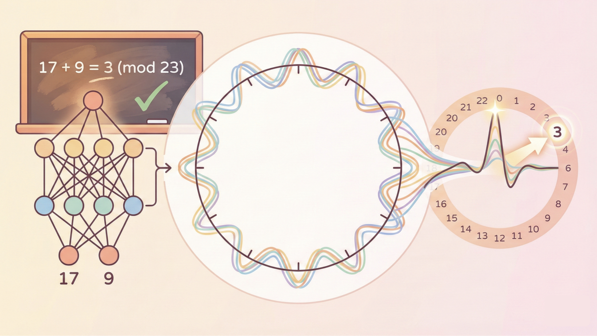
Cover Figure: A two-layer neural network (left) learns to compute $17 + 9 = 3 \pmod{23}$ by discovering Fourier features: each hidden neuron becomes a cosine wave at a single frequency (center). These waves, spread symmetrically with different phases and at different frequencies, combine into a “majority vote” that peaks sharply at the correct answer on the modular number line (right).
Abstract
We present a comprehensive analysis of how two-layer neural networks learn features to solve the modular addition task. Our work provides a full mechanistic interpretation of the learned model and a theoretical explanation of its training dynamics. While prior work has identified that individual neurons learn single-frequency Fourier features and phase alignment, it does not fully explain how these features combine into a global solution. We bridge this gap by formalizing a diversification condition that emerges during training when overparametrized, consisting of two parts: phase symmetry and frequency diversification. We prove that these properties allow the network to collectively approximate a flawed indicator function on the correct logic for the modular addition task. While individual neurons produce noisy signals, the phase symmetry enables a majority-voting scheme that cancels out noise, allowing the network to robustly identify the correct sum. Furthermore, we explain the emergence of these features under random initialization via a lottery ticket mechanism. Our gradient flow analysis proves that frequencies compete within each neuron, with the “winner” determined by its initial spectral magnitude and phase alignment. From a technical standpoint, we provide a rigorous characterization of the layer-wise phase coupling dynamics and formalize the competitive landscape using the ODE comparison lemma. Finally, we use these insights to demystify grokking, characterizing it as a three-stage process involving memorization followed by two generalization phases, driven by the competition between loss minimization and weight decay.
1. Introduction and Motivation
Modular addition has emerged as a canonical testbed for this program. The task is deceptively simple: given two integers $x$ and $y$ drawn from $\{0, 1, \ldots, p-1\}$ (where $p$ is a prime), predict their sum modulo $p$. There is no noise, no ambiguity, just pure arithmetic in a cyclic group. Yet when a neural network is trained on this task, the solution it discovers is anything but trivial. The network does not learn a lookup table. Instead, it spontaneously discovers Fourier features, the mathematical structures that underlie harmonic analysis on cyclic groups. How and why this happens is the subject of our paper.
Prior work has made important progress on pieces of this puzzle. Nanda et al. (2023) used mechanistic interpretability to show that one-layer transformers trained on modular addition learn Fourier features, and introduced progress measures to track grokking. Zhong et al. (2023) identified a “clock” and “pizza” representation in the embedding space. Power et al. (2022) first discovered the grokking phenomenon itself. Liu et al. (2022) and Morwani et al. (2023) studied the margin-maximization landscape for algebraic tasks. However, these works leave three major questions open:
Our paper provides the first unified answers to all three questions. We work with a two-layer fully-connected network, the simplest architecture that can learn the task, because its transparency allows complete inspection of every weight and every computation.
2. Setup and Summary of Results
The Modular Addition Task
Given two integers $x, y \in \mathbb{Z}_p = \{0, 1, \ldots, p-1\}$ (where $p$ is a prime, typically $p = 23$ in our experiments), predict:
$$z = (x + y) \bmod p.$$For concreteness: with $p = 23$, the input $(17, 9)$ should produce the output $26 \bmod 23 = 3$. The complete dataset has $p^2 = 529$ examples, every possible pair $(x, y)$. There is no noise; the task is purely deterministic.
Two-Layer Neural Network Model
We use a two-layer fully-connected neural network with $M = 512$ hidden neurons and no bias terms. Each input integer $x$ is represented as a one-hot vector $e_x \in \mathbb{R}^p$. The network computes a logit vector $f(x,y) \in \mathbb{R}^p$:
$$f(x, y) = \sum_{m=1}^{M} \xi_m \cdot \sigma\bigl(\theta_m[x] + \theta_m[y]\bigr),$$where $\theta_m \in \mathbb{R}^p$ is the input weight of neuron $m$ (the notation $\theta_m[x]$ looks up the $x$-th entry of $\theta_m$), $\xi_m \in \mathbb{R}^p$ is the output weight, and $\sigma$ is the activation function (ReLU in experiments, quadratic $\sigma(x) = x^2$ for theory).
The network is trained to minimize the cross-entropy loss (equivalently, the negative log-likelihood under softmax). For each input pair $(x,y)$, let $j^* = (x+y) \bmod p$ denote the correct answer. The loss over dataset $\mathcal{D}$ is:
$$\ell_{\mathcal{D}}(\xi, \theta) = \sum_{(x,y) \in \mathcal{D}} \left[ -f(x,y;\xi,\theta)[j^*] + \log \sum_{j=0}^{p-1} \exp\bigl(f(x,y;\xi,\theta)[j]\bigr) \right],$$which has a clean interpretation: the first term pushes up the logit of the correct answer, while the log-sum-exp term penalizes all logits, preventing them from growing unchecked. We optimize using AdamW with learning rate $\eta = 10^{-4}$.
Training Setups
We study the model under two training setups:
Full-data setup (Parts I-II: Mechanism and Dynamics). Following prior work (Morwani et al., 2023; Tian et al., 2024), we train on the complete dataset $\mathcal{D}_{\text{full}}$ of all $p^2$ input pairs, without train-test splitting and without weight decay. This yields more stable training dynamics and cleaner learned features, making it easier to study the mechanism and dynamics.
Train-test split setup (Part III: Grokking). Following prior work (Nanda et al., 2023), which identifies train-test splitting and weight decay as key factors for inducing grokking, we randomly partition the dataset using a training fraction of 0.75 and apply a weight decay of 2.0. These two ingredients (incomplete data + weight decay) are the standard conditions for inducing grokking.
Summary of Results
Our results answer three questions. We summarize each below; the rest of the blog unpacks each one in depth.
Q1. The Mechanism: How does the trained network compute modular addition?
We show that the trained model effectively approximates an indicator function via a majority-voting scheme in Fourier space. After training, each neuron’s weights form a cosine at a single Fourier frequency $k$, with an input phase $\phi$ and an output phase $\psi = 2\phi$ (we call this phase alignment). Each neuron individually produces a noisy, biased signal. But the 512 neurons collectively satisfy a full diversification condition: they cover all $(p-1)/2$ frequencies with balanced magnitudes and uniformly spread phases. Under this condition, the network aggregates the biased signals into a collective approximation of the indicator $\mathbf{1}(x + y \equiv j \bmod p)$. The true-signal peak at the correct answer $j = (x+y) \bmod p$ exceeds spurious peaks at $2x \bmod p$ and $2y \bmod p$ by a margin of $aNp/8$, so the softmax output concentrates on the correct sum.
Q2. The Dynamics: How do Fourier features emerge from random initialization?
We explain the emergence of these features via a lottery ticket mechanism. Under small initialization, the gradient flow decouples across neurons and across frequency components within each neuron, reducing to independent four-variable ODEs per (neuron, frequency) pair. Each neuron’s input weight has a phase $\phi$ (the horizontal shift of its cosine pattern) and its output weight has a phase $\psi$. The quantity $\mathcal{D} = (2\phi - \psi) \bmod 2\pi$, called the phase misalignment, measures how far the two layers are from cooperating coherently. Our analysis proves that frequencies compete within each neuron, with the winner determined by its initial spectral magnitude and phase alignment. The frequency with the smallest initial misalignment aligns first, and super-linear positive feedback compounds its advantage, suppressing all competitors. Perhaps the most striking consequence: the final trained predictor is entirely determined by the random initialization, before a single gradient step is taken.
Q3. Grokking: Why does the network generalize long after memorization?
We characterize grokking as a three-stage process driven by the competition between loss minimization and weight decay. Stage I (Memorization): The loss gradient dominates, and a “perturbed” lottery runs on incomplete data (75% of pairs), producing a rough Fourier solution that memorizes training examples but does not generalize. We also identify a common-to-rare ordering: the network first memorizes symmetric pairs while actively suppressing rare ones. Stage II (Fast Generalization): Weight decay prunes non-feature frequencies, sharpening the noisy representation into a clean single-frequency-per-neuron structure. Test accuracy jumps sharply. Stage III (Slow Cleanup): The loss gradient vanishes and weight decay alone gently shrinks all norms, polishing the solution to perfect test accuracy.
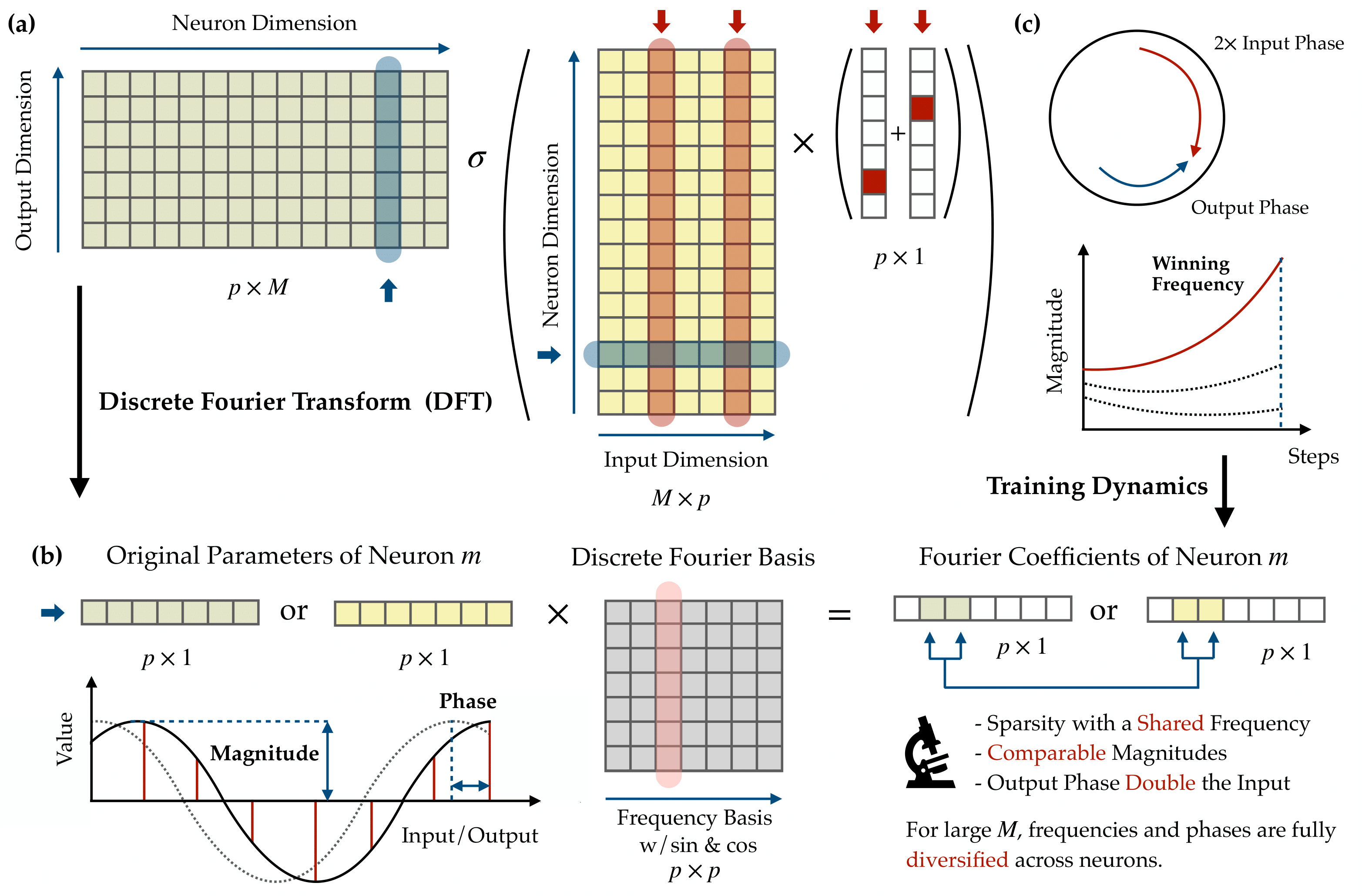 Figure 1. An illustration of our primary analytical technique and results. (a) The neural network architecture: a two-layer fully connected network takes one-hot encoded inputs $x, y \in \mathbb{R}^p$, passes them through $M$ neurons with activation $\sigma(\cdot)$, and produces a logit vector in $\mathbb{R}^p$. We apply the Discrete Fourier Transform (DFT) to each neuron’s input and output weight vectors, decomposing them into Fourier coefficients, a magnitude and phase per frequency. (b) The DFT in action on a single neuron: the raw weight vector (left) is projected onto the discrete Fourier basis of sine and cosine waves (center), yielding a sparse set of Fourier coefficients (right). After training, each neuron’s energy concentrates at a single frequency, so the weights are well-described by a single cosine with a definite magnitude and phase. (c) Key mechanistic interpretability findings. Top: Phase alignment, where the output phase $\psi_m$ locks to exactly twice the input phase $\phi_m$ ($\psi = 2\phi$), ensuring coherent signal production. Bottom: The lottery ticket mechanism during training, where multiple frequencies compete within each neuron, but only one (the “winning frequency,” determined by the smallest initial phase misalignment) grows explosively while all others are suppressed. The bottom text summarizes the collective properties: sparsity at a shared frequency, comparable magnitudes across neurons, the doubled-phase relationship, and full diversification when the network is wide.
3. Part I: The Mechanism — What the Trained Network Computes
After training the network to 100% accuracy on the full dataset, we inspect the learned weights. The findings are striking: the network has independently discovered the Discrete Fourier Transform.
3.1 Empirical Observations
We make four key observations about the structure of the trained network. Each observation is stated as a finding, supported by figures, and then explained intuitively.
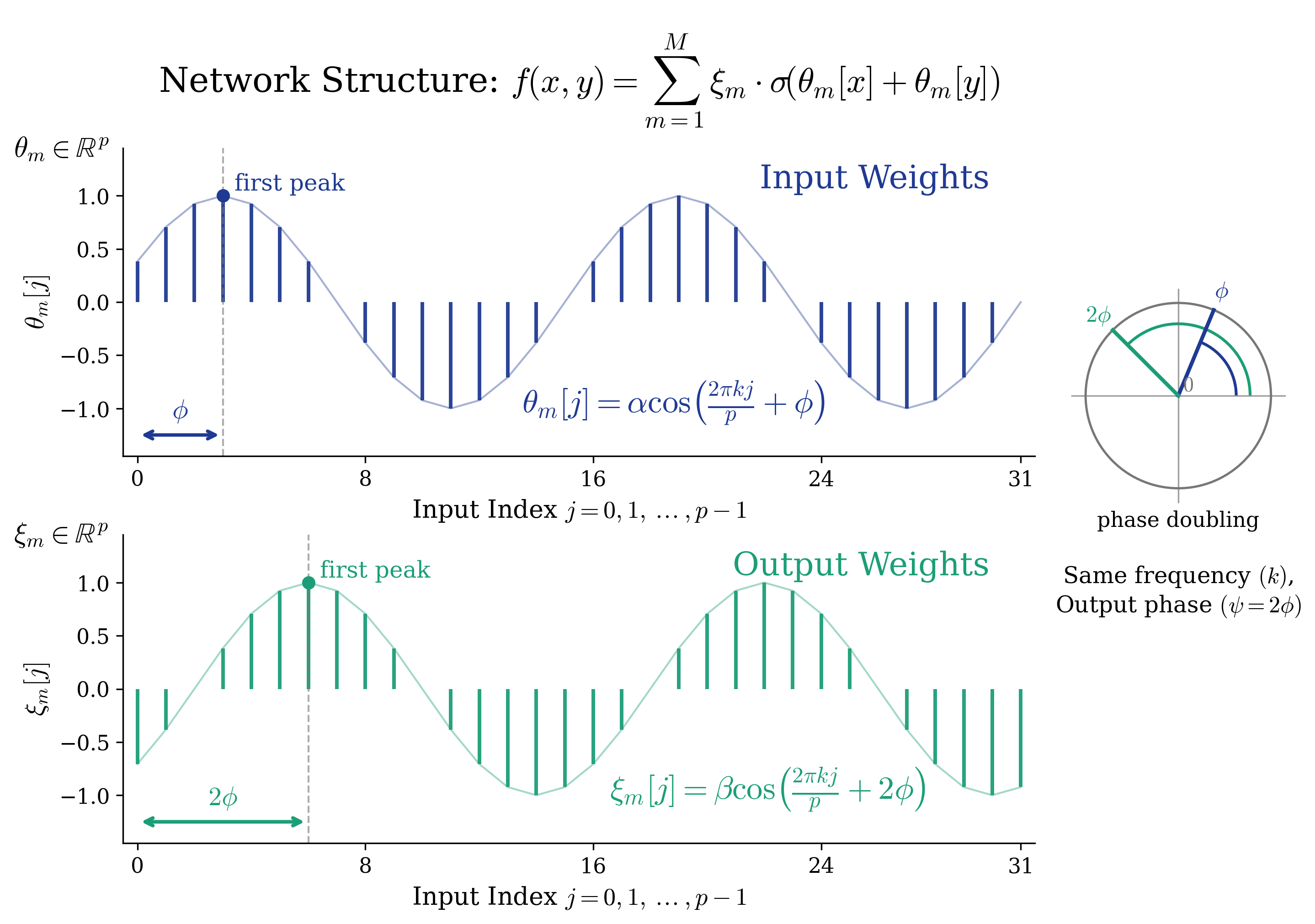
Figure 2. Anatomy of a single trained neuron: cosine weights and phase doubling. After training, each neuron $m$ in the two-layer network $f(x,y) = \sum_m \xi_m \cdot \sigma(\theta_m[x] + \theta_m[y])$ develops a striking structure. Top: the input weight vector $\theta_m \in \mathbb{R}^p$ traces a clean cosine curve $\alpha \cos(2\pi k j / p + \phi)$ at a single frequency $k$, with input phase $\phi$. Bottom: the output weight vector $\xi_m \in \mathbb{R}^p$ is also a cosine at the same frequency $k$, but its phase is exactly doubled: $\psi = 2\phi$ (green arrow), as illustrated by the polar diagram on the right. These two properties — single-frequency cosine structure (Observation 1) and the $\psi = 2\phi$ phase alignment (Observation 2) — are the building blocks of the network’s Fourier-based algorithm for modular addition.
Observation 1: Every Neuron is a Cosine Wave (Fourier Features)
When we plot the entries of a trained neuron’s input weight vector $\theta_m[j]$ against $j = 0, 1, \ldots, p-1$, the result is a clean cosine curve:
$$\theta_m[j] = \alpha_m \cos\!\left(\frac{2\pi k}{p} \cdot j + \phi_m\right), \qquad \xi_m[j] = \beta_m \cos\!\left(\frac{2\pi k}{p} \cdot j + \psi_m\right).$$Each neuron has:
- A single active frequency $k$ (out of the $(p-1)/2 = 11$ possible nonzero frequencies for $p = 23$).
- An input magnitude $\alpha_m$ and input phase $\phi_m$.
- An output magnitude $\beta_m$ and output phase $\psi_m$.
No one told the network about Fourier analysis — it reinvented this representation from scratch through gradient descent.
To verify this, we apply the Discrete Fourier Transform (DFT) to each neuron’s weight vector and plot the result as a heatmap. Each row corresponds to a neuron, and each column to a Fourier mode (cosine and sine components for each frequency $k$). The result is sparse: every neuron concentrates its energy at a single frequency, with all other frequencies essentially zero.
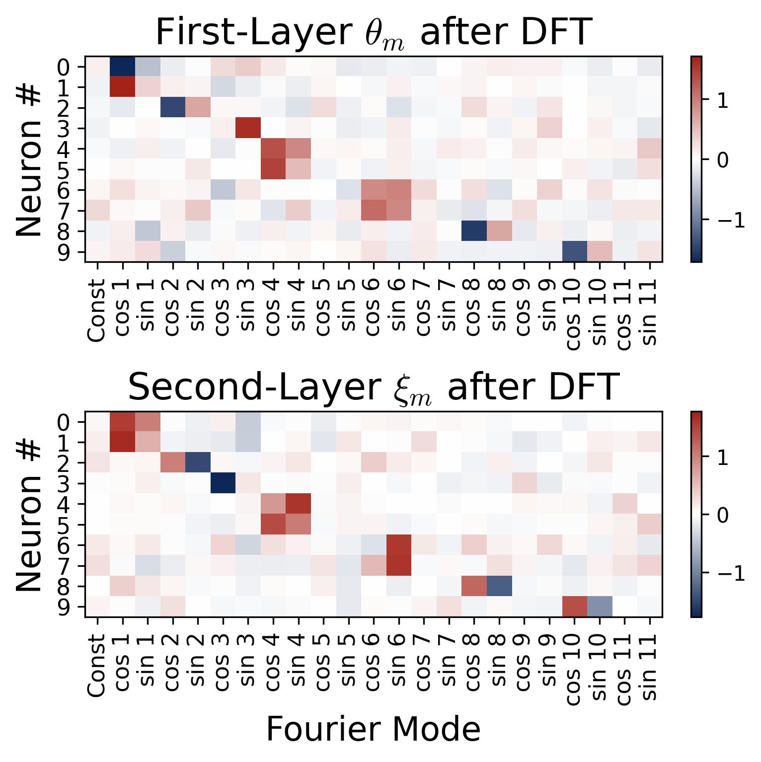
Figure 3. Fourier sparsity of learned weights (10 representative neurons). We apply the Discrete Fourier Transform to each neuron’s weight vector and display the result as a heatmap. Each row is one of the first 10 neurons (out of 512 total); each column is a Fourier mode (cosine and sine components for frequencies $k = 1, \ldots, 11$); color indicates the DFT coefficient value. Each neuron concentrates virtually all its energy at a single frequency, visible as one bright cell per row, with all other entries near zero. Note that this 10-neuron sample shows only a subset of the 11 available frequencies; the remaining frequencies are represented by neurons not shown here. The same single-frequency pattern holds across all 512 neurons, with the full population covering all 11 nonzero frequencies for $p = 23$ (see Observation 3 on collective diversification).
We can also verify the cosine structure by fitting cosine curves directly to the raw weight vectors. The fits are nearly perfect:
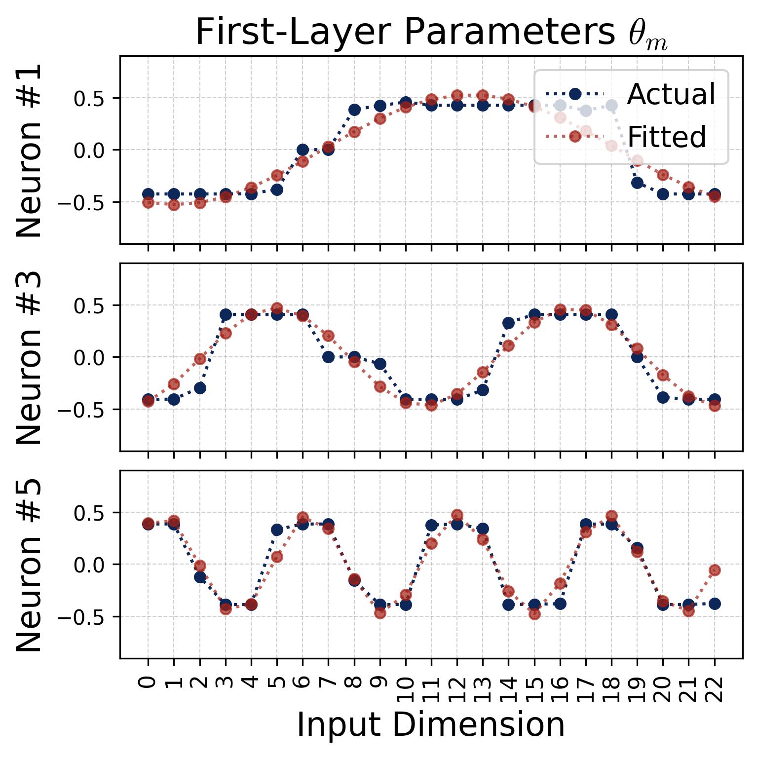
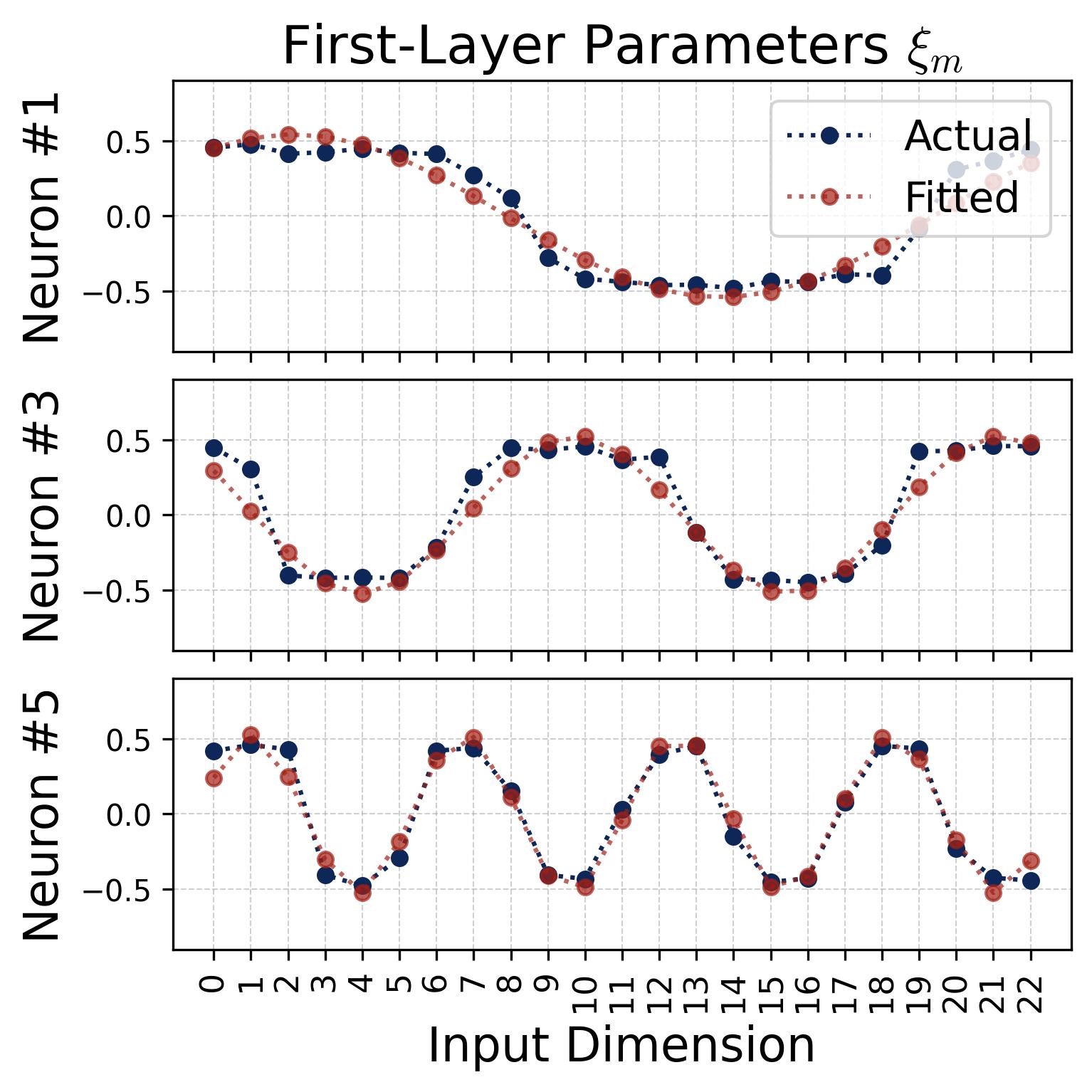
Figure 4. Cosine fits to individual neurons. For several representative neurons, we plot the raw learned weight values (blue dots/curves) against the index $j = 0, 1, \ldots, p-1$ and overlay a best-fit cosine of the form $a \cdot \cos(\omega_k j + \phi)$ (red dashed curves), where $a$ and $\phi$ are the fitted magnitude and phase. Left: input weights $\theta_m[j]$. Right: output weights $\xi_m[j]$. The fits are nearly perfect (residuals are negligible), confirming that each neuron’s weight vector is well-described by a single cosine at one Fourier frequency. Different neurons fit to different frequencies $k$ and different phases $\phi_m$, $\psi_m$, consistent with the diversification described in Observation 3.
Observation 2: Phase Alignment — The Doubled-Phase Relationship
The input phase $\phi_m$ and output phase $\psi_m$ are not independent — they satisfy a precise relationship:
$$\psi_m = 2\phi_m \pmod{2\pi}.$$If we scatter-plot $(2\phi_m \bmod 2\pi,\; \psi_m \bmod 2\pi)$ across all 512 neurons, every point falls on the diagonal line $y = x$.
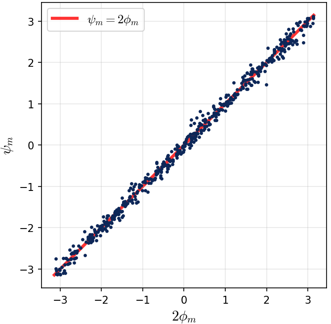
Figure 5. Phase alignment between input and output layers. Each dot represents one of the 512 neurons, plotted at coordinates $(2\phi_m \bmod 2\pi,\; \psi_m \bmod 2\pi)$, where $\phi_m$ is the input-layer phase and $\psi_m$ is the output-layer phase. Every point falls precisely on the diagonal $y = x$, confirming the doubled-phase relationship $\psi_m = 2\phi_m$. This coupling is not imposed by architecture or initialization — it is learned through training. As we show theoretically, it arises because the quadratic (even) activation produces terms proportional to $\cos(\omega_k j + 2\phi_m)$, and the output layer aligns its phase to match, creating a coherent signal that peaks at the correct answer $(x+y) \bmod p$.
Why “doubled phase”? To see why the factor of 2 is natural, consider what happens when the network computes $\sigma(\theta_m[x] + \theta_m[y])$. With a quadratic (or more generally, even) activation, squaring the sum of two cosines produces terms involving the sum of their phases. Since both the $x$ and $y$ inputs use the same weight vector $\theta_m$ (and hence the same phase $\phi_m$), the product formula $\cos(A)\cos(B) = \frac{1}{2}[\cos(A+B) + \cos(A-B)]$ naturally generates terms involving $2\phi_m$. The output layer “locks onto” this by setting $\psi_m = 2\phi_m$, ensuring that the input and output layers work coherently to produce a signal that peaks at $(x + y) \bmod p$.
Observation 3: Collective Diversification
When the network is wide enough ($M = 512 \gg (p-1)/2 = 11$ frequencies), the neurons organize themselves into a balanced, symmetric ensemble with three properties:
- Frequency balance. Every frequency $k \in \{1, \ldots, 11\}$ is represented by roughly the same number of neurons.
- Phase uniformity. Within each frequency group, the input phases $\phi_m$ are approximately uniformly distributed around the circle $(-\pi, \pi)$.
- Magnitude homogeneity. The products $\alpha_m \beta_m^2$ are nearly identical across neurons — no single neuron dominates the output.
This collective organization is not enforced by any explicit constraint in the training objective. It emerges spontaneously because it is the configuration that minimizes noise in the majority-voting mechanism (as we will explain in Section 4.2).
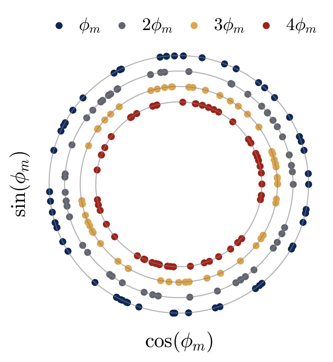
Figure 6. Higher-order phase symmetry within a frequency group. For a single frequency group $\mathcal{N}_k$ (all neurons sharing the same dominant frequency $k$), we plot the phase angles $\iota \cdot \phi_m \bmod 2\pi$ on concentric polar rings for $\iota = 1, 2, 3, 4$. Each dot is one neuron. The near-uniform spacing around every ring confirms that the phases satisfy the symmetry conditions $\sum_m e^{i \cdot \iota \cdot \phi_m} \approx 0$ for $\iota = 2, 4$ — the exact conditions required for noise cancellation in the majority-voting mechanism. Without this symmetry, the phase-dependent noise terms would persist and the network could not achieve perfect accuracy. The network learns this symmetric configuration spontaneously.
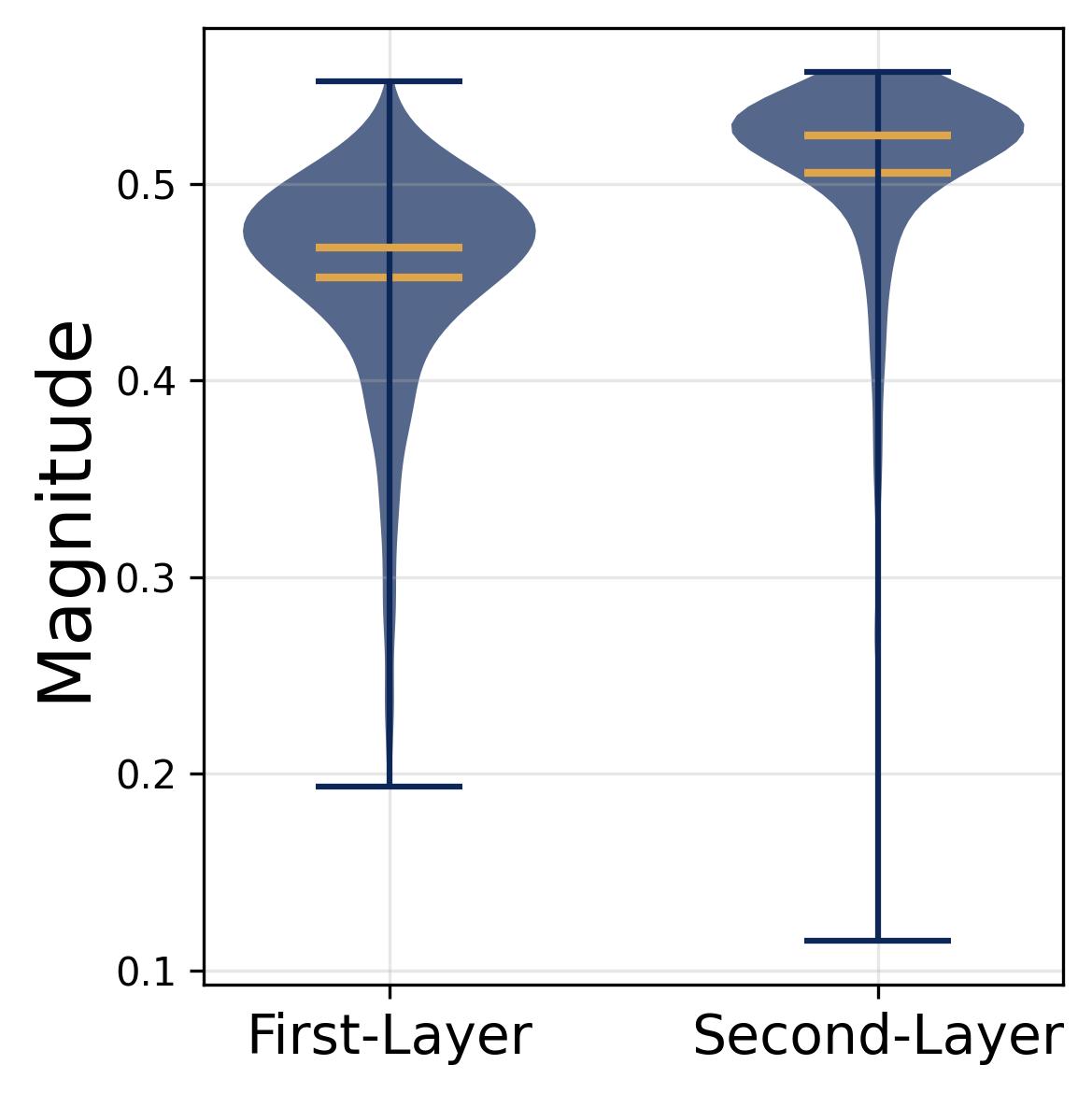
Figure 7. Magnitude homogeneity across neurons. Violin plots of the learned input magnitudes $\alpha_m$ and output magnitudes $\beta_m$ across all 512 neurons. Both distributions are tightly concentrated around their respective means, with very little spread. This confirms Observation 3(c): no single neuron dominates the network’s output. Magnitude homogeneity ensures that each neuron’s “vote” in the majority-voting mechanism carries roughly equal weight, preventing any one neuron from biasing the result. Combined with frequency balance and phase uniformity, this completes the full diversification condition required for exact noise cancellation.
The phase uniformity condition can be stated formally: for each frequency group $\mathcal{N}_k = \{m : \text{neuron } m \text{ uses frequency } k\}$ and for $\iota \in \{2, 4\}$,
$$\sum_{m \in \mathcal{N}_k} e^{i \cdot \iota \cdot \phi_m} \approx 0.$$This is the condition that causes the noise terms in the majority-voting mechanism to cancel.
Observation 4: Activation Robustness — Only the Even Part Matters
Here is a revealing experiment: take a model trained with ReLU and, at test time, replace the activation with something else. The results:
| Activation at test time | $\|x\|$ | $x^2$ | $x^4$ | $\log(1+e^{2x})$ | $e^x$ | $x$ | $x^3$ |
|---|---|---|---|---|---|---|---|
| Accuracy | 100% | 100% | 100% | 100% | 100% | 4.1% | 3.6% |
Any activation with a nonzero even component works perfectly. Purely odd activations ($x$, $x^3$) fail completely.
Why this happens. Recall that $\mathrm{ReLU}(x) = \frac{1}{2}(x + |x|)$, which decomposes into an odd part ($\frac{1}{2}x$) and an even part ($\frac{1}{2}|x|$). Under the phase symmetry of Observation 3, the odd part’s contribution cancels across neurons (because $\sum_m \cos(\omega_k j + \phi_m) \approx 0$ by phase uniformity), leaving only the even part. This means the network’s solution is not specific to ReLU — it works for any activation with a nonzero even component. This observation justifies our use of the quadratic activation $\sigma(x) = x^2$ for theoretical analysis: it is the simplest even activation and produces the same qualitative behavior as ReLU.
3.2 The Mechanism: Majority Voting in Fourier Space
Now that we know what the neurons look like, we can work out how they combine to produce the correct answer.
What a Single Neuron Computes
With quadratic activation and the phase-alignment condition $\psi_m = 2\phi_m$, a single neuron’s contribution to the output logit at position $j$ takes the form:
$$f^{[m]}(x,y)[j] \;\propto\; \cos^2\!\left(\frac{\omega_k(x-y)}{2}\right) \cdot \biggl[\underbrace{\cos\bigl(\omega_k(x+y-j)\bigr)}_{\text{signal}} + \;\underbrace{2\cos(\omega_k j + 2\phi_m) + \cos\bigl(\omega_k(x+y+j) + 4\phi_m\bigr)}_{\text{noise}}\biggr],$$where $\omega_k = 2\pi k / p$ is the $k$-th Fourier frequency.
Let us read this formula carefully:
- The signal term $\cos(\omega_k(x+y-j))$ is maximized when $j = (x+y) \bmod p$, because $\cos(0) = 1$. This is the term that “knows” the correct answer.
- The noise terms depend on the neuron’s phase $\phi_m$ (through $2\phi_m$ and $4\phi_m$). Their sign and magnitude vary from neuron to neuron.
- The prefactor $\cos^2(\omega_k(x-y)/2)$ depends on $x - y$ rather than $x + y$. This is the structural “Achilles’ heel” — it modulates the signal in a way that cannot be eliminated by diversification, because it does not depend on the neuron’s phase $\phi_m$. When we sum over neurons, this prefactor factors out as a common multiplier for every neuron in the frequency group.
A single neuron’s vote is biased: it points toward the correct answer but is contaminated by noise that depends on its particular frequency-phase combination. The critical question is whether aggregating many such biased votes can recover the correct answer.
Noise Cancellation through Diversification
The answer is yes, provided the neurons are fully diversified (Observation 3). When we sum the single-neuron contributions over all neurons in frequency group $\mathcal{N}_k$, the $\cos^2$ prefactor factors out (since it is independent of $\phi_m$), and we are left with:
$$\sum_{m \in \mathcal{N}_k} f^{[m]} \;\propto\; \cos^2\!\left(\frac{\omega_k(x-y)}{2}\right) \cdot \Bigl[N \cdot \cos(\omega_k(x+y-j)) \;+\; \underbrace{2\!\sum_m \cos(\omega_k j + 2\phi_m)}_{= \;0 \text{ by } \iota=2 \text{ symmetry}} \;+\; \underbrace{\sum_m \cos(\omega_k(x+y+j) + 4\phi_m)}_{= \;0 \text{ by } \iota=4 \text{ symmetry}}\Bigr].$$The signal term $\cos(\omega_k(x+y-j))$ adds coherently ($N$ identical copies), while the noise terms cancel by the phase symmetry conditions of Observation 3. After cancellation, each frequency group contributes:
$$\sum_{m \in \mathcal{N}_k} f^{[m]} \;\propto\; \cos^2\!\left(\frac{\omega_k(x-y)}{2}\right) \cdot \cos(\omega_k(x+y-j)).$$From the Prefactor to Spurious Peaks
The $\cos^2$ prefactor is the source of the spurious peaks. To see how, expand it using $\cos^2(\theta) = \frac{1}{2}(1 + \cos(2\theta))$:
$$\cos^2\!\left(\frac{\omega_k(x-y)}{2}\right) = \frac{1}{2}\bigl(1 + \cos(\omega_k(x-y))\bigr).$$Substituting this back, the contribution from frequency group $k$ becomes two terms (up to proportionality):
$$\cos^2\!\left(\frac{\omega_k(x-y)}{2}\right) \cdot \cos(\omega_k(x+y-j)) \;=\; \frac{1}{2}\cos(\omega_k(x+y-j)) \;+\; \frac{1}{2}\cos(\omega_k(x-y))\cos(\omega_k(x+y-j)).$$The first term is a clean signal that depends on $x+y-j$. The second term involves $\cos(\omega_k(x-y))$, which we expand using the product-to-sum identity $\cos(A)\cos(B) = \frac{1}{2}[\cos(A+B) + \cos(A-B)]$:
$$\cos(\omega_k(x-y))\cos(\omega_k(x+y-j)) = \frac{1}{2}\bigl[\cos(\omega_k(2x - j)) + \cos(\omega_k(2y - j))\bigr].$$So the per-frequency contribution splits into three cosine sums (up to proportionality):
$$\frac{1}{2}\cos(\omega_k(x+y-j)) \;+\; \frac{1}{4}\cos(\omega_k(2x-j)) \;+\; \frac{1}{4}\cos(\omega_k(2y-j)).$$Now we sum over all frequency groups $k = 1, \ldots, (p-1)/2$ and apply the Fourier identity
$$\sum_{k=1}^{(p-1)/2} \cos(\omega_k z) = \frac{p}{2} \cdot \mathbf{1}(z \equiv 0 \bmod p) - \frac{1}{2},$$which follows from the orthogonality of characters on $\mathbb{Z}_p$: the full sum $\sum_{k=0}^{p-1} e^{i\omega_k z} = p \cdot \mathbf{1}(z \equiv 0 \bmod p)$, and taking the real part and exploiting the symmetry $\cos(\omega_k z) = \cos(\omega_{p-k} z)$ to fold the sum in half gives the identity above.
to each of the three cosine sums. Each sum collapses into an indicator function, giving the final result.
Majority-Voting Approximates the Indicator Function
Proposition 1 (Mechanism). Suppose the neurons are completely diversified. Under the cosine parametrization and phase alignment $2\phi_m - \psi_m = 0 \bmod 2\pi$, the output logit at dimension $j$ takes the form:
$$f(x,y)[j] = \frac{aN}{2}\left[-1 + \frac{p}{2}\cdot\mathbf{1}(x+y \equiv j \bmod p) + \frac{p}{4}\cdot\bigl(\mathbf{1}(2x \equiv j \bmod p) + \mathbf{1}(2y \equiv j \bmod p)\bigr)\right],$$where $a = \alpha_m \beta_m^2$ is the common magnitude product across all neurons (by the homogeneous scaling condition of full diversification) and $N$ is the number of neurons per frequency group. The overall scale $a$ grows during training as the network’s weights increase in norm, which progressively sharpens the softmax output toward the correct answer. The constant $-1$ collects the three $-\frac{1}{2}$ terms from the Fourier identity applied to the three cosine sums ($-\frac{1}{2} - \frac{1}{4} - \frac{1}{4} = -1$).
The first indicator $\mathbf{1}(x+y \equiv j)$ is the correct answer, with coefficient $p/2$. The remaining two indicators are spurious peaks at $j = 2x \bmod p$ and $j = 2y \bmod p$, each with coefficient $p/4$. These spurious peaks are a direct consequence of the “Achilles’ heel” prefactor $\cos^2(\omega_k(x-y)/2)$: the $\cos(\omega_k(x-y))$ term inside the expansion mixes $x$ and $y$ into $2x$ and $2y$ via the product-to-sum identity, and the Fourier sum then converts these cosines into indicator functions at the wrong locations.
A Worked Example: $p = 23$, $x = 3$, $y = 7$
The correct answer is $(3 + 7) \bmod 23 = 10$. The spurious peaks appear at $2 \times 3 \bmod 23 = 6$ and $2 \times 7 \bmod 23 = 14$.
| Output index $j$ | What fires | Logit (relative to $aN/2$) |
|---|---|---|
| $j = 10$ | Correct answer $(3+7 = 10)$ | $-1 + 23/2 = \mathbf{+10.5}$ |
| $j = 6$ | Spurious peak $(2 \times 3 = 6)$ | $-1 + 23/4 = +4.75$ |
| $j = 14$ | Spurious peak $(2 \times 7 = 14)$ | $-1 + 23/4 = +4.75$ |
| All other $j$ | Background | $-1$ |
The correct answer always has the largest logit, with a margin of $p/4 = 5.75$ over the spurious peaks. The softmax then amplifies this gap exponentially:
$$\mathrm{softmax}(f)[j_{\text{correct}}] \geq 1 - (p-1) \cdot e^{-aNp/8} \approx 1.$$Since the magnitudes $a$ grow during training, the network naturally achieves this condition, and the softmax output converges to a perfect one-hot vector.
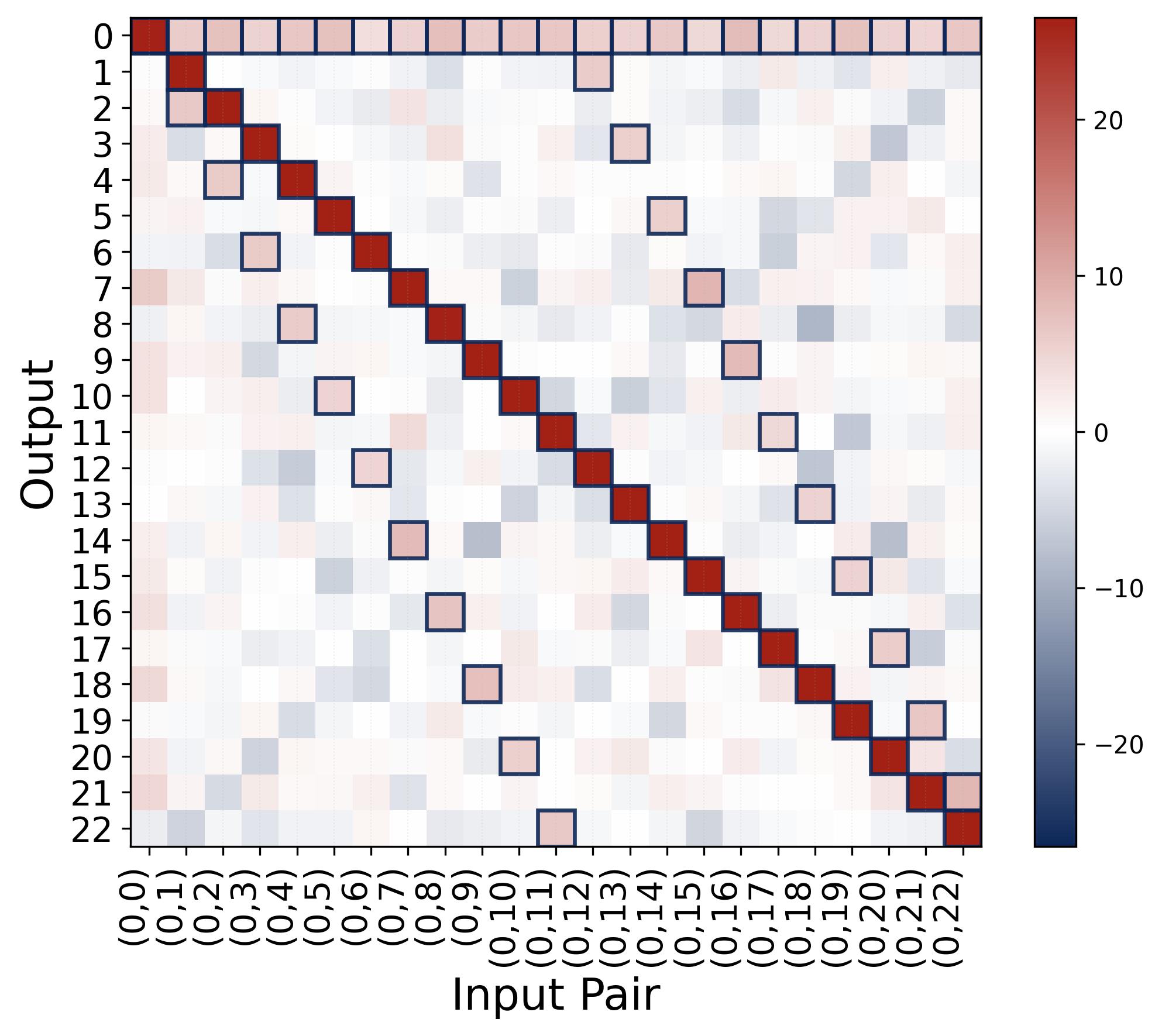
Figure 8. Output logits confirm the indicator-function structure. The heatmap shows the output logit $f(x, y)[j]$ for fixed $x = 0$ and all $y \in \{0, \ldots, 22\}$ (columns) versus output index $j$ (rows), with $p = 23$ and quadratic activation. The bright red diagonal marks the correct answer $j = (0 + y) \bmod 23 = y$, which receives the highest logit (around $+25$). For example, at input $(0, 5)$, the brightest cell is at output $j = 5$. The faint pink cells (marked by small boxes) are the spurious peaks predicted by Proposition 1, located at $j = 2x \bmod 23 = 0$ (a persistent faint row along output 0) and $j = 2y \bmod 23$ (a secondary diagonal; for input $(0, 5)$, this appears at output $j = 10$). These spurious peaks have logits roughly half as large as the correct answer (approximately $aNp/8$ vs. $aNp/4$). The visible color difference between the bright red correct cells and the faint pink spurious cells reflects the margin of $aNp/8$ that separates them. The softmax amplifies this gap exponentially, turning even a modest margin into near-certain predictions. All remaining cells are near the background level (blue/white, around $-aN/2$).
Summary of the mechanism. The trained network implements a three-step computation: (1) each neuron encodes inputs as cosine waves at a single frequency; (2) the quadratic (even) activation produces a noisy vote for the correct answer; (3) diversification across neurons cancels the noise via destructive interference, producing an approximation to the indicator function that softmax sharpens into a correct prediction. This is a majority vote in Fourier space.
4. Part II: Training Dynamics — How Features Emerge
We now turn to the deeper question: how does the network arrive at this elegant Fourier structure starting from random initialization? The answer involves two key theoretical results, single-frequency preservation (the lottery ticket mechanism) and phase alignment dynamics, both derived by analyzing the gradient flow of the loss function.
4.1 The Fourier Lens
The natural coordinate system for understanding modular addition is the Fourier basis on $\mathbb{Z}_p$. The Fourier basis is natural here because $\mathbb{Z}_p$ is a cyclic group under addition modulo $p$, and the Fourier basis diagonalizes convolutions on cyclic groups. Using the Discrete Fourier Transform, each neuron $m$’s weight vectors can be decomposed exactly as:
$$\theta_m[j] = \alpha_m^0 + \sum_{k=1}^{(p-1)/2} \alpha_m^k \cdot \cos(\omega_k j + \phi_m^k), \qquad \xi_m[j] = \beta_m^0 + \sum_{k=1}^{(p-1)/2} \beta_m^k \cdot \cos(\omega_k j + \psi_m^k),$$where $\theta_m$ is the input weight vector and $\xi_m$ is the output weight vector. For each frequency $k$, the magnitudes $\alpha_m^k, \beta_m^k > 0$ control the amplitude and the phases $\phi_m^k, \psi_m^k \in [-\pi, \pi)$ control the horizontal shift. This decomposition is exact and holds for any parameter vector; the key empirical finding (Observation 1) is that training drives all but one frequency to zero, so only a single $k$ survives per neuron.
4.2 Neuron and Frequency Decoupling
The first theoretical insight is that, under small initialization ($\kappa_{\text{init}} \ll 1$), the training dynamics simplify dramatically through two levels of decoupling.
Neuron decoupling. When all parameters are small, the softmax output is approximately uniform: $\mathrm{softmax}(f(x,y))[j] \approx 1/p$. This approximation makes the gradient of the log-partition function (the second component of the cross-entropy loss) independent of the specific weights, causing all inter-neuron coupling terms to vanish. Each neuron then evolves according to its own gradient, independently of all other neurons.
Frequency decoupling. Within each neuron, the gradient computation involves sums of the form $\sum_{x \in \mathbb{Z}_p} \cos(\omega_k x) \cos(\omega_\tau x)$. By the orthogonality of characters on $\mathbb{Z}_p$:
$$\sum_{x \in \mathbb{Z}_p} \cos(\omega_k x) \cos(\omega_\tau x) = \frac{p}{2} \cdot \delta_{k,\tau},$$so cross-frequency terms vanish whenever $k \neq \tau$. This is the fundamental reason why different frequencies evolve independently: the cyclic group structure of modular addition ensures that Fourier modes are orthogonal.
The result is that the full dynamics of the entire network reduce to independent copies of a four-variable ODE, one for each (neuron, frequency) pair.
4.3 The Four-Variable ODE
For a single frequency $k$ within neuron $m$, dropping indices for clarity, the dynamics take the form:
$$\partial_t \alpha \approx 2p \cdot \alpha \cdot \beta \cdot \cos(\mathcal{D}),$$$$\partial_t \beta \approx p \cdot \alpha^2 \cdot \cos(\mathcal{D}),$$$$\partial_t \mathcal{D} \approx -p\cdot(4\beta^2-\alpha^2/\beta) \cdot \sin(\mathcal{D}),$$where $\mathcal{D} = (2\phi - \psi) \bmod 2\pi$ is the phase misalignment.
This system has a clear physical interpretation:
Magnitudes grow when phases are aligned. The growth rates $\partial_t \alpha$ and $\partial_t \beta$ are proportional to $\cos(\mathcal{D})$. When $\mathcal{D} \approx 0$ (good alignment), $\cos(\mathcal{D}) \approx 1$ and magnitudes grow rapidly. When $\mathcal{D} < \pi/2$ (poor alignment), $\cos(\mathcal{D}) < 0$ and magnitudes decrease.
Phases rotate toward alignment. The phase velocities are proportional to $\sin(\mathcal{D})$, with opposite signs for $\phi$ and $\psi$. Both $2\phi$ and $\psi$ converge toward each other, driving $\mathcal{D} \to 0$.
Self-reinforcing dynamics. As alignment improves, magnitudes grow faster. But the phase dynamics slow down (since $\sin(\mathcal{D}) \to 0$). The system naturally coordinates: phases align first (while magnitudes are small), then magnitudes explode.
4.4 Phase Alignment: The Zero-Attractor
Theorem (Phase Alignment). The phase misalignment $\mathcal{D}(t) = (2\phi(t) - \psi(t)) \bmod 2\pi$ converges to zero from any initial condition (except the measure-zero unstable point $\mathcal{D} = \pi$).
The dynamics of $\mathcal{D}$ on the circle behave like an overdamped pendulum: $\mathcal{D} = 0$ is a stable attractor and $\mathcal{D} = \pi$ is an unstable repeller. To see why:
- When $\mathcal{D} \in (0, \pi)$, we have $\sin(\mathcal{D}) > 0$, and the combined effect of $\partial_t \phi$ and $\partial_t \psi$ rotates $\mathcal{D}$ clockwise toward 0.
- When $\mathcal{D} \in (\pi, 2\pi)$, we have $\sin(\mathcal{D}) < 0$, and the sign flip ensures counterclockwise rotation, again toward 0.
This result explains Observation 2 (the doubled-phase relationship $\psi = 2\phi$): it is not a coincidence or a special property of the initialization, but an inevitable consequence of the training dynamics. The gradient flow actively drives the phases into alignment.
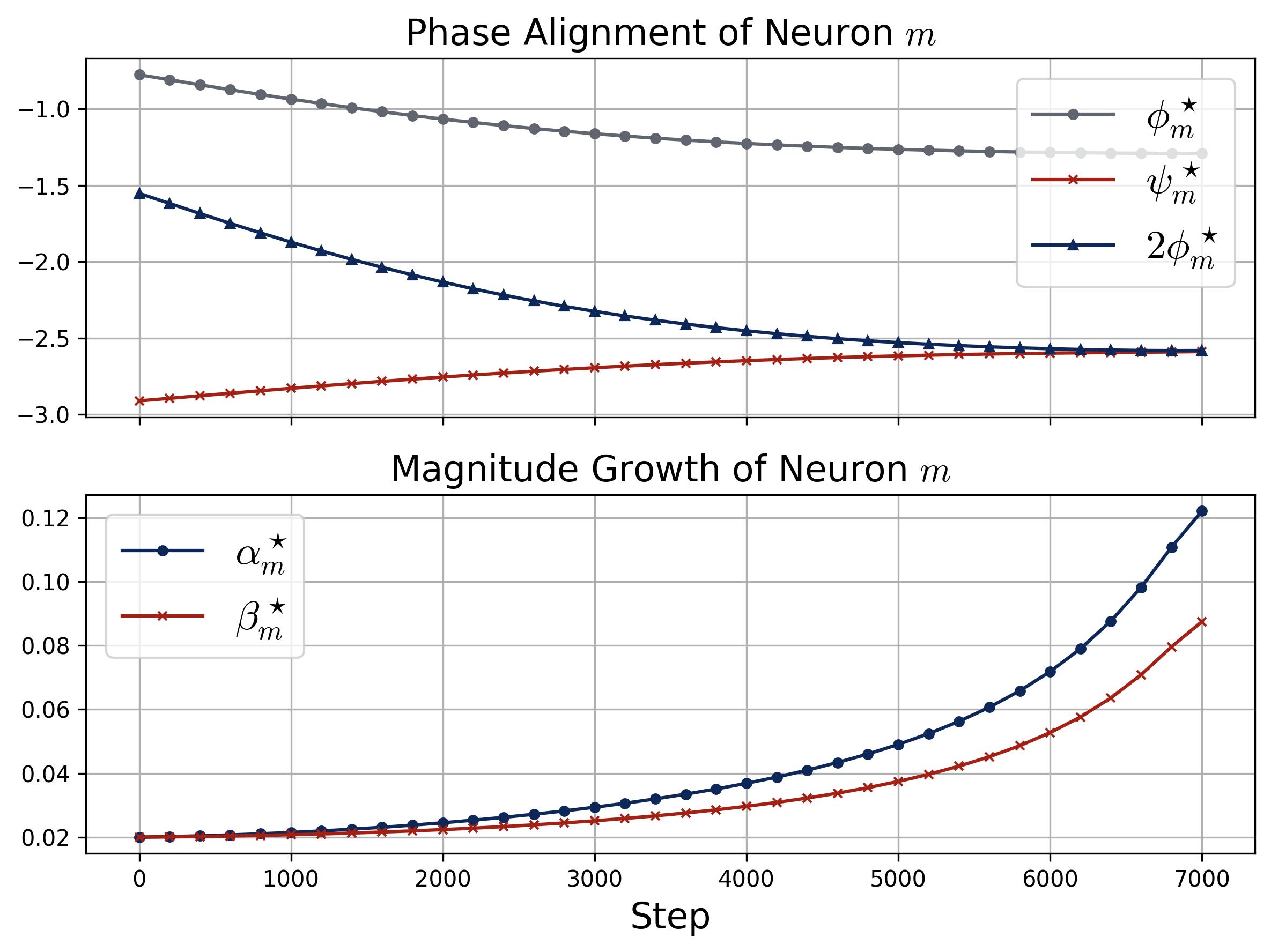
Figure 9. Phase alignment and magnitude growth for a single neuron. Two stacked panels track the dynamics of a specific neuron $m$ during training (quadratic activation, $\kappa_{\text{init}} = 0.02$). Top (Phase Alignment): Three curves show $\phi_m^\star$ (gray), $\psi_m^\star$ (red), and $2\phi_m^\star$ (dark blue with triangles) over training steps. The key observation is that $2\phi_m^\star$ and $\psi_m^\star$ converge toward each other, confirming that the phase misalignment $\mathcal{D}_m^\star = (2\phi_m^\star - \psi_m^\star) \bmod 2\pi$ is driven to zero, exactly as predicted by the zero-attractor ODE. Bottom (Magnitude Growth): The input magnitude $\alpha_m^\star$ (blue) and output magnitude $\beta_m^\star$ (red) both start at $\kappa_{\text{init}} = 0.02$ and remain nearly flat while the phases are still misaligned, then accelerate rapidly once alignment is achieved (around step 4,000). This confirms the self-reinforcing loop: alignment enables growth, and growth accelerates alignment.
4.5 Single-Frequency Preservation and the Lottery Ticket
Theorem (Single-Frequency Preservation). Under the decoupled gradient flow, if a neuron starts at a single-frequency state (energy concentrated at one frequency $k^\star$), it remains at that single-frequency state for all time.
This result follows directly from frequency decoupling: since different frequencies evolve independently, a frequency that starts at zero magnitude stays at zero forever.
But at initialization, neurons have energy at all frequencies (random initialization distributes energy uniformly across the Fourier spectrum). So why does each neuron end up with a single frequency?
The lottery ticket mechanism. At initialization, each frequency $k$ within neuron $m$ starts with the same small magnitude $\kappa_{\text{init}}$ but a random phase misalignment $\mathcal{D}_m^k(0)$. The magnitude ODE shows that the growth rate of frequency $k$ on neuron $m$ is proportional to $\cos(\mathcal{D}_m^k(t))$: when the phase misalignment is small, $\cos(\mathcal{D}_m^k) \approx 1$ and the magnitude grows rapidly; when misalignment is large, growth stalls. The frequency that starts with the smallest misalignment (the best “lottery ticket”) aligns fastest, and once aligned, its magnitude begins to grow explosively. This creates positive feedback: better alignment accelerates growth, and larger magnitudes in turn speed up alignment, so once the leading frequency pulls ahead, the gap compounds exponentially. The other frequencies on the same neuron, having larger initial misalignment, never get the chance to align and their magnitudes remain near $\kappa_{\text{init}}$, effectively frozen out by the winner’s dominance. The winner takes all.
Corollary (Lottery Ticket). The winning frequency for neuron $m$ is:
$$k^\star = \arg\min_k \widetilde{\mathcal{D}}_m^k(0),$$where $\widetilde{\mathcal{D}}_m^k(0)$ is the initial phase misalignment. The dominance time scales as $\widetilde{O}(\log p / (p \kappa_{\text{init}}))$.
Since the initial misalignments are independent and uniformly distributed, different neurons generically select different winning frequencies. With enough neurons ($M \gg (p-1)/2$), all frequencies are covered, explaining Observation 1 (single-frequency structure) and contributing to Observation 3 (frequency balance).
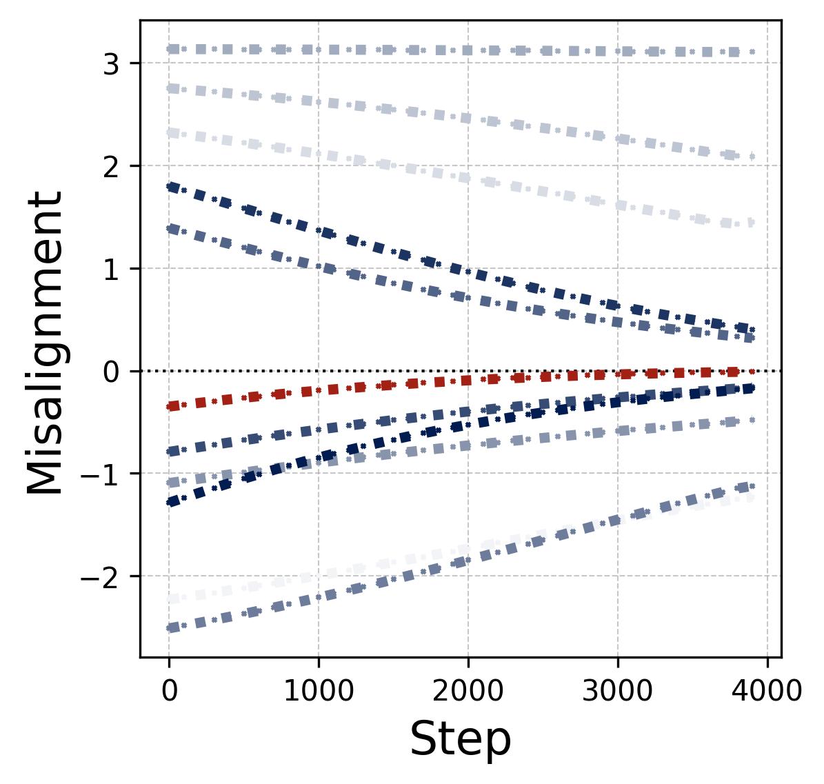
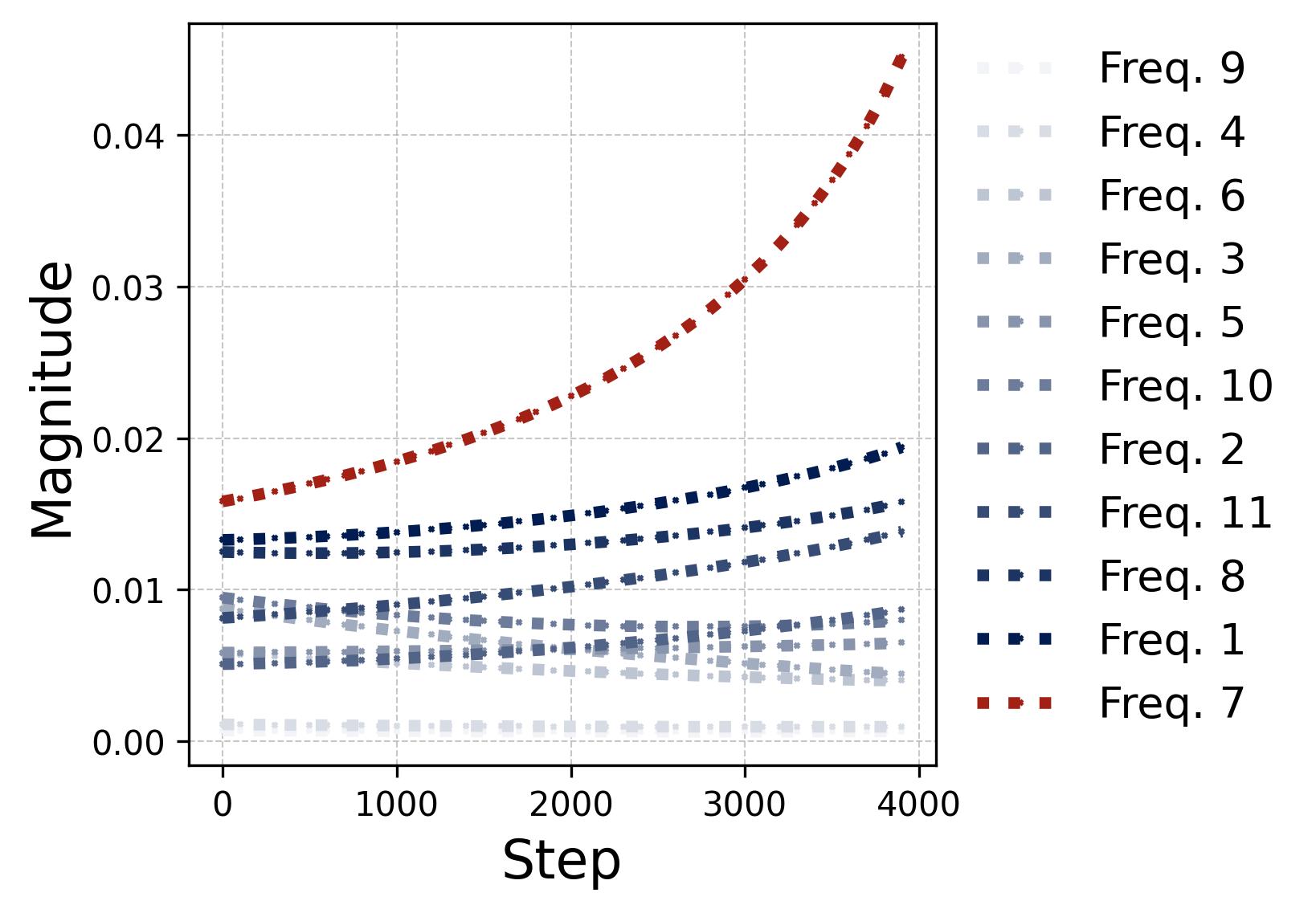
Figure 10. The lottery ticket race within a single neuron. We track all $(p-1)/2 = 11$ frequency components within one neuron during training under random initialization. Left (phase misalignment): Each curve shows $\mathcal{D}_m^k(t) = (2\phi_m^k - \psi_m^k) \bmod 2\pi$ (rescaled to $[-\pi, \pi)$) for a different frequency $k$. The winning frequency (Freq. 7, highlighted in red) starts with the smallest initial misalignment and converges to $\mathcal{D} = 0$ fastest. The losing frequencies drift slowly but their alignment does not matter because their magnitudes never grow large enough to compete. Right (magnitudes): The corresponding output magnitude $\beta_m^k(t)$ for each frequency. The legend is sorted by initial magnitude. Once the winning frequency’s phase aligns ($\mathcal{D} \approx 0$), its magnitude undergoes explosive super-linear growth (visible as the red curve pulling away after step 1,000), while all other frequencies grow only slowly and remain far below the winner. This is the positive feedback loop: better alignment leads to faster growth, which in turn accelerates alignment. The winner is determined at initialization by the combination of initial magnitude and initial phase misalignment.
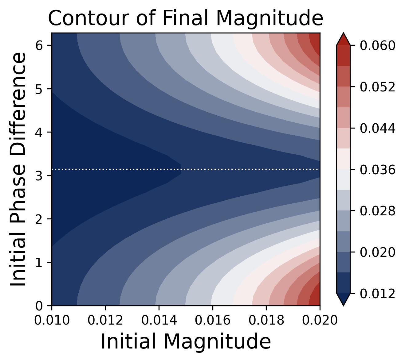
Figure 11. Outcome of the lottery as a function of initial conditions. Contour plot showing the final learned magnitude $\beta_m^k$ (color) as a function of two initial-condition variables: the initial magnitude $\beta_m^k(0)$ (horizontal axis) and the initial phase misalignment $\mathcal{D}_m^k(0)$ (vertical axis). The largest final magnitudes (brightest region, bottom-right) correspond to frequencies that start with large initial magnitude and small phase misalignment — the “winning lottery tickets." The contours are symmetric about $\mathcal{D} = \pi$, confirming that only the distance $|\mathcal{D} - 0|$ (not its sign) determines the outcome. Frequencies starting near $\mathcal{D} = \pi$ (the dotted horizontal line at the center of the y-axis) achieve negligible final magnitude regardless of their initial size, because they are trapped near the unstable fixed point before escaping and aligning.
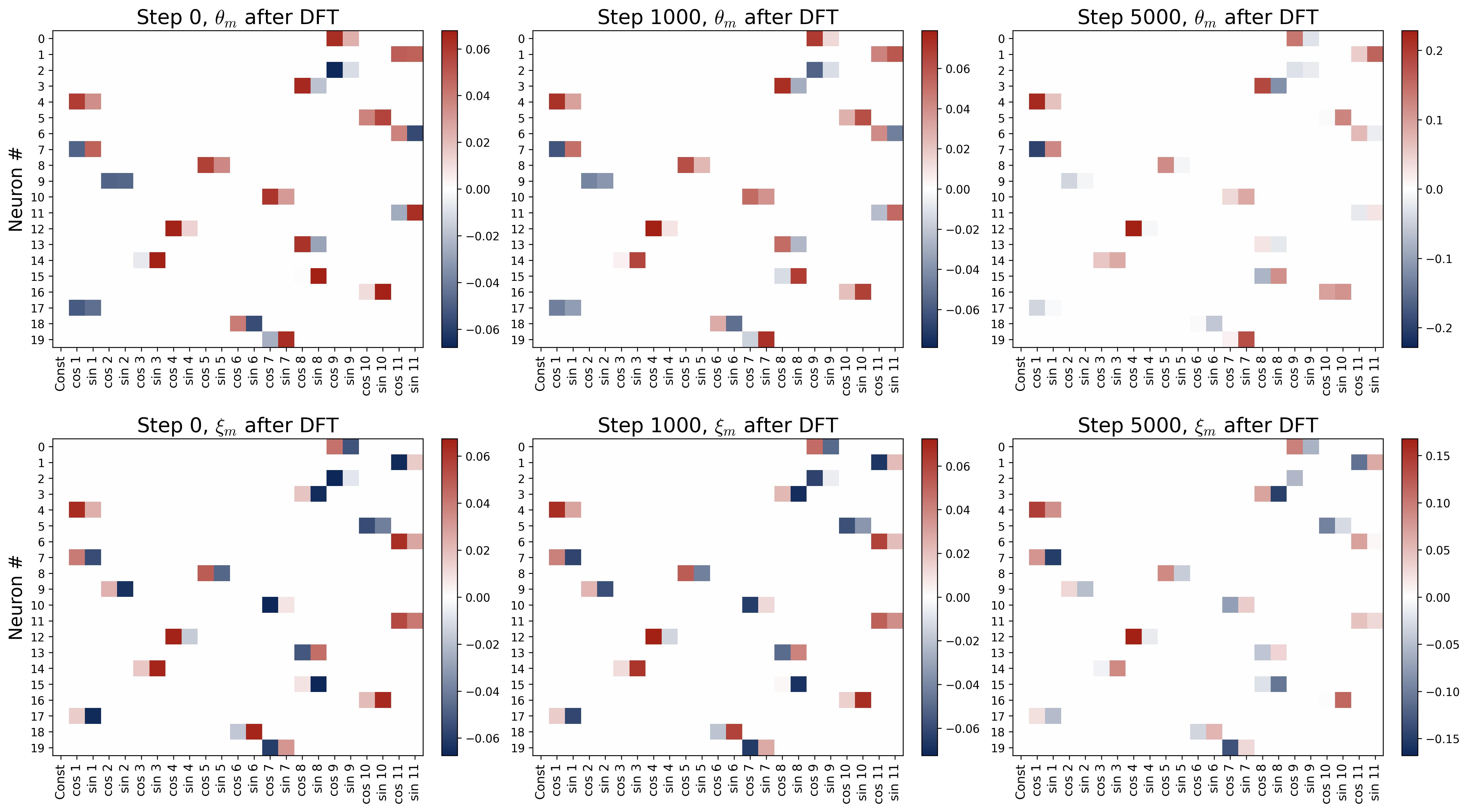
Figure 12. Single-frequency preservation under quadratic activation. Six panels in a 2×3 grid show the DFT heatmaps at three training snapshots (Step 0, Step 1000, Step 5000). Top row: input weights $\theta_m$; bottom row: output weights $\xi_m$. Rows are neurons; columns are Fourier modes. Each neuron is initialized with all its energy at a single frequency $k^\star$ (per Assumption 1). At Step 0, each neuron has exactly one bright cell at its assigned frequency. At Steps 1000 and 5000, these bright cells grow in intensity while all other frequency entries remain at zero, confirming our Theorem (Single-Frequency Preservation): under the decoupled gradient flow with quadratic activation, the Fourier support of each neuron’s weights is preserved exactly. No energy leaks between modes.
4.6 Beyond Quadratic: ReLU Dynamics
The theoretical analysis above uses the quadratic activation for tractability, but in practice networks are trained with ReLU. The key finding is that all the qualitative phenomena carry over: single-frequency concentration, phase alignment, and the lottery ticket mechanism all occur under ReLU, with only minor quantitative differences. The main distinction is a small amount of energy “leakage” to harmonic multiples of the dominant frequency. A harmonic multiple of a frequency $k^\star$ is simply an integer multiple $2k^\star, 3k^\star, 5k^\star, \ldots$ (taken modulo $p$), analogous to overtones in acoustics. For the input weights, energy leaks to odd harmonics ($3k^\star$, $5k^\star$, $\ldots$); for the output weights, energy leaks to all harmonics ($2k^\star$, $3k^\star$, $\ldots$). The leakage decays quadratically with the harmonic order: the third harmonic has $1/9$ the strength of the dominant frequency, the fifth harmonic has $1/25$, and so on, keeping the dominant frequency overwhelmingly dominant. We refer readers to the paper for the formal analysis.
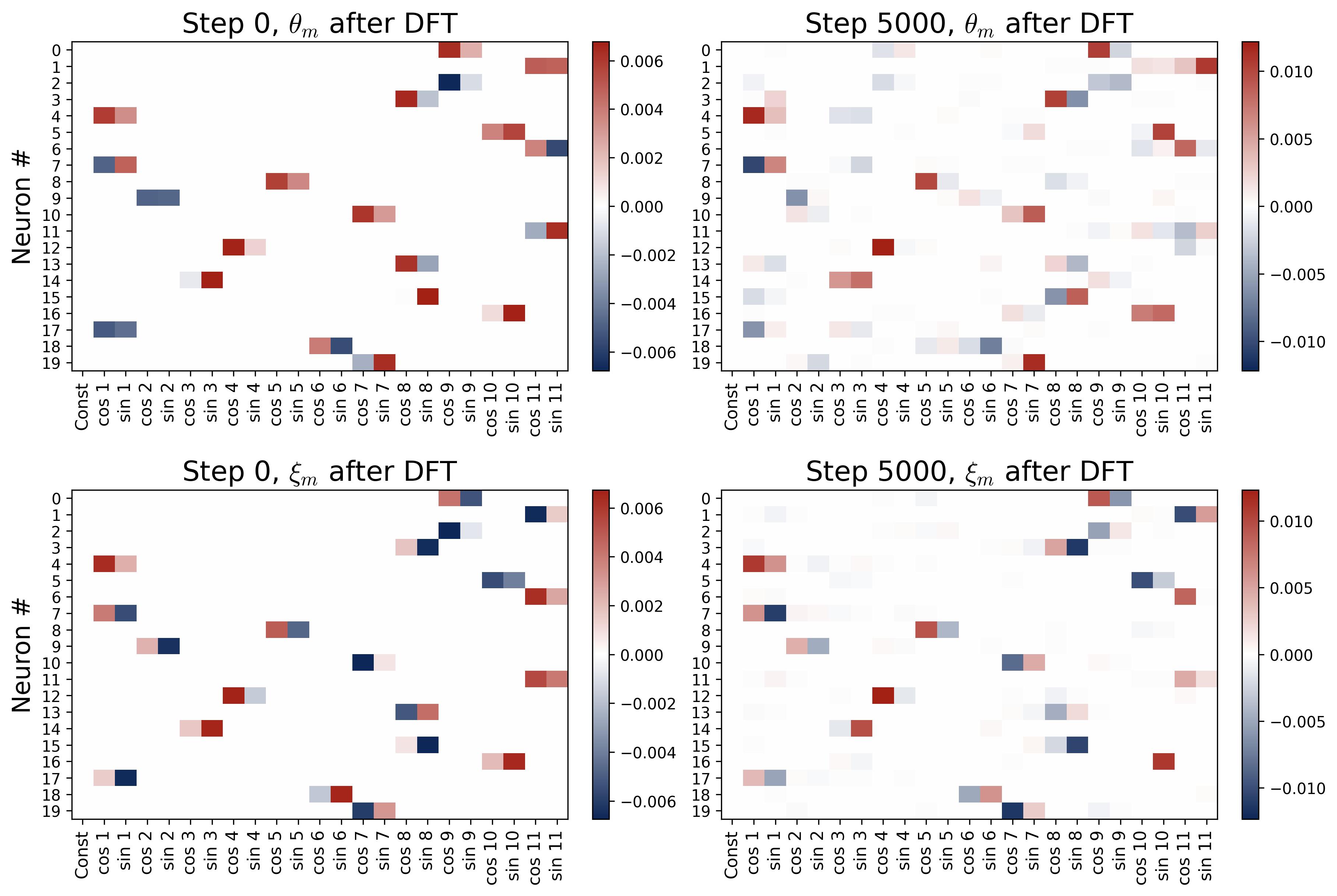
Figure 13a. Approximate single-frequency preservation under ReLU. Four panels in a 2×2 grid show DFT heatmaps of the first 20 neurons at initialization (Step 0, left) and after training (Step 5000, right), with input weights $\theta_m$ on top and output weights $\xi_m$ on bottom. Unlike the perfectly clean quadratic case (Figure 12), training with ReLU produces small but visible energy at harmonic multiples of the dominant frequency $k^\star$ (e.g., at $3k^\star$ and $5k^\star$ for $\theta_m$, and at $2k^\star$ and $3k^\star$ for $\xi_m$). However, the dominant frequency remains overwhelmingly dominant: the third harmonic has only $1/9$ the strength, the fifth only $1/25$, and so on.
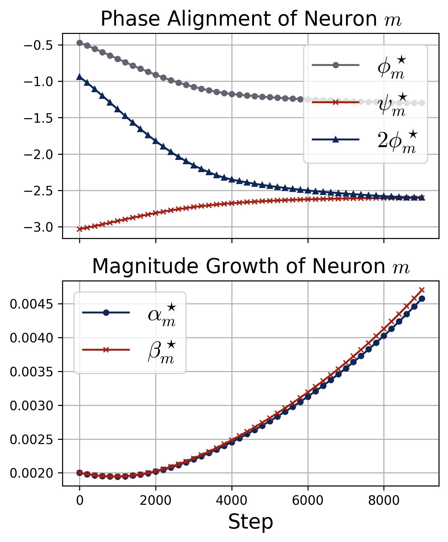
Figure 13b. Phase alignment and magnitude growth under ReLU. Same layout as Figure 9 but with ReLU activation. Top: The three phase curves ($\phi_m^\star$, $\psi_m^\star$, and $2\phi_m^\star$) converge so that $2\phi_m^\star \to \psi_m^\star$, confirming that the zero-attractor behavior holds under ReLU with only minor quantitative differences (alignment takes longer, ~8,000 steps vs. ~5,000 for quadratic). Bottom: The magnitudes $\alpha_m^\star$ and $\beta_m^\star$ remain flat until phases align, then accelerate, following the same pattern as the quadratic case. This confirms that the quadratic theory captures the essential dynamics of ReLU training.
5. Part III: Grokking — From Memorization to Generalization
We now turn to the most dramatic phenomenon: grokking. Under the train-test split setup (75% training data, weight decay of 2.0; see Section 2), a striking pattern emerges: the network quickly memorizes the training set, achieving 100% training accuracy, but then takes much longer (often orders of magnitude more training steps) to generalize to the held-out test set. This delayed generalization is grokking.
Our analysis, built on the understanding of the mechanism and dynamics from the previous sections, reveals that grokking is not a single mysterious event but a three-stage process, each stage driven by a different balance of forces.
5.1 Overview of the Three Stages
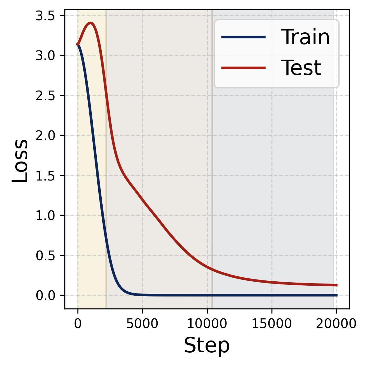
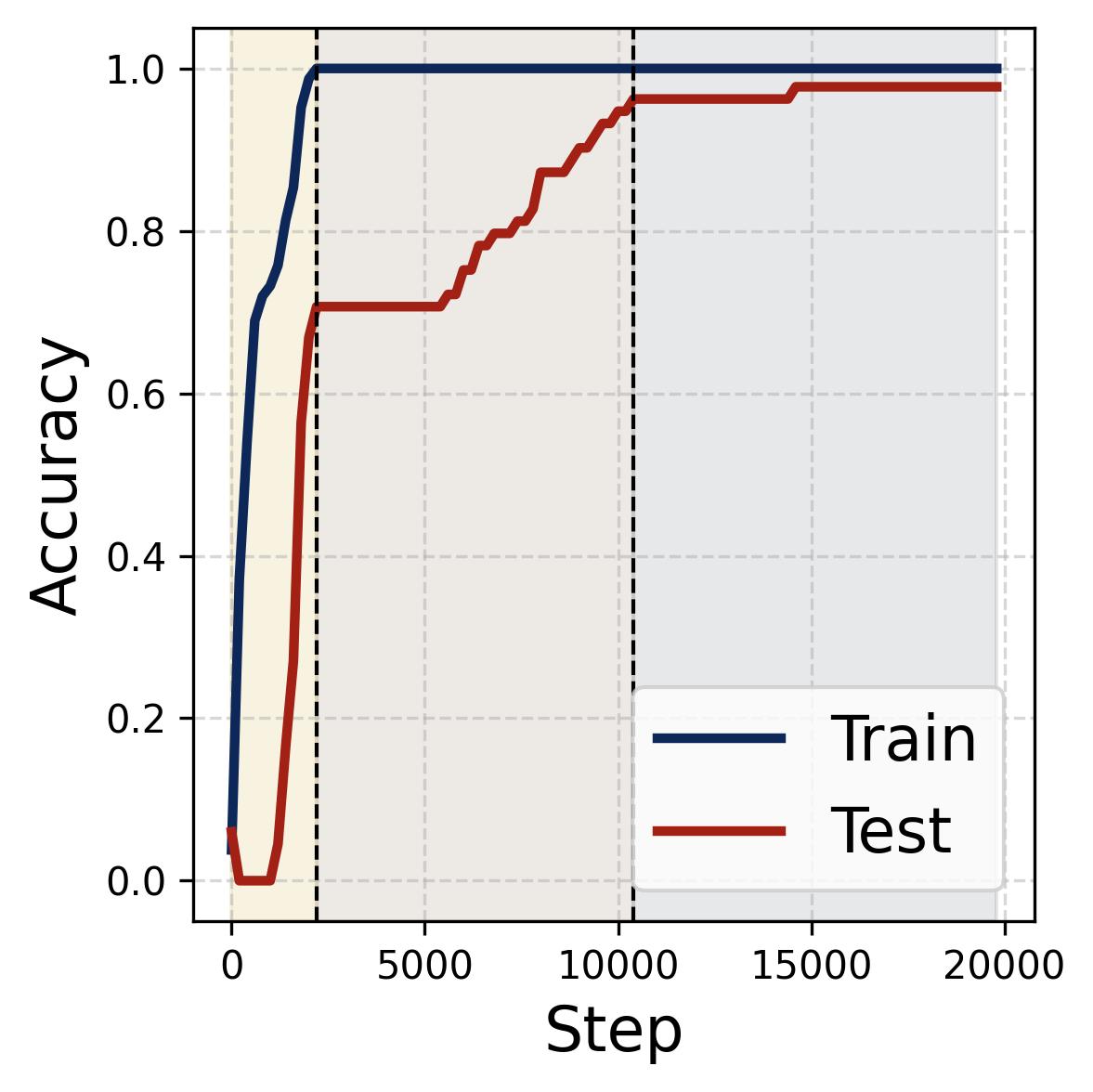
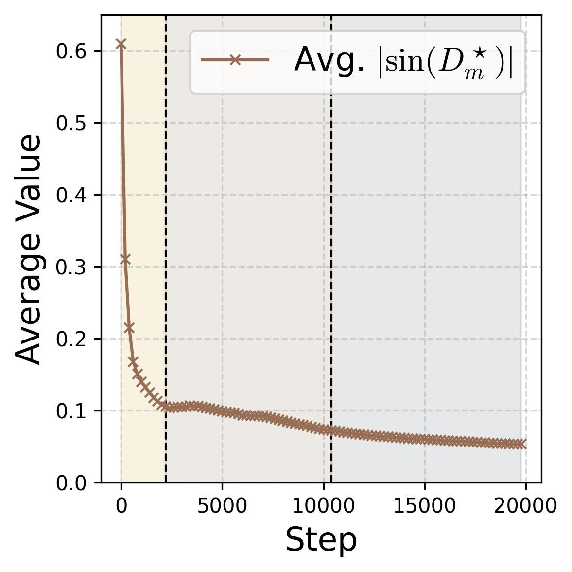
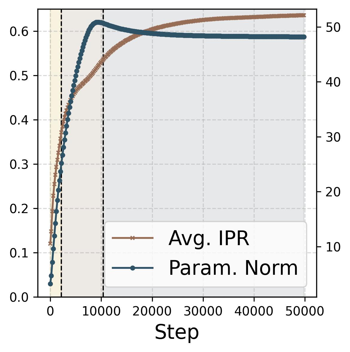
Figure 14. Four progress measures reveal the three stages of grokking. The network is trained on 75% of all $(x,y)$ pairs with weight decay $\lambda = 2.0$. The three colored background regions (yellow, tan, gray) correspond to the three stages, separated by dashed vertical lines at ~2,200 and ~10,000 steps. (a) Loss: Training loss (dark blue) drops rapidly to near zero within the first ~2,000 steps (Stage I), while test loss (dark red) remains high, then drops sharply during Stage II and slowly decays during Stage III. (b) Accuracy: Training accuracy (dark blue) reaches 100% early; test accuracy (dark red) plateaus at ~70% during memorization (because the symmetric architecture gives “free” accuracy on $(y,x)$ pairs), then climbs to ~95% during Stage II, and converges toward 100% during Stage III. (c) Phase alignment: The average $|\sin(\mathcal{D}_m^\star)|$ (measuring misalignment of the dominant frequency’s phases) decreases throughout, confirming that phase alignment continues to improve even after memorization. (d) Frequency sparsity (IPR) and parameter norm: The average IPR (brown, left axis; higher = sparser) increases throughout training as neurons concentrate energy at fewer frequencies. The parameter norm (dark blue, right axis) grows rapidly during Stages I-II when the loss gradient dominates, then plateaus and slightly decreases once weight decay takes over in Stage III.
5.2 Stage I: Memorization (Loss Minimization Dominates)
In the first stage, the loss gradient dominates and the network rapidly memorizes the training data. Training accuracy reaches 100% while test accuracy reaches only about 70%.
Why ~70% and not ~50%? The model’s architecture is symmetric in $x$ and $y$: the input is $\theta_m[x] + \theta_m[y]$, which is invariant under swapping $(x, y) \leftrightarrow (y, x)$. This means that if the model correctly classifies $(x, y)$, it automatically gets $(y, x)$ right. Since the training set includes roughly 75% of all pairs, many test pairs $(y, x)$ have their symmetric counterpart $(x, y)$ in the training set, giving “free” test accuracy.
The perturbed lottery. During this stage, the lottery ticket mechanism runs, but on incomplete data. The missing test pairs perturb the Fourier orthogonality that drives frequency decoupling, producing a “noisy” version of the single-frequency solution. A dominant frequency emerges (visible in the DFT heatmaps), but energy persists at other frequencies because the data does not cover all of $\mathbb{Z}_p^2$.
Common-to-rare memorization. Within the memorization stage, we observe a fascinating ordering: the network first memorizes common input pairs (those where both $(i, j)$ and $(j, i)$ are in the training set) and then memorizes rare pairs where only one ordering appears. During the first sub-phase, the network actually suppresses performance on rare examples, actively driving their accuracy to zero before eventually memorizing them.
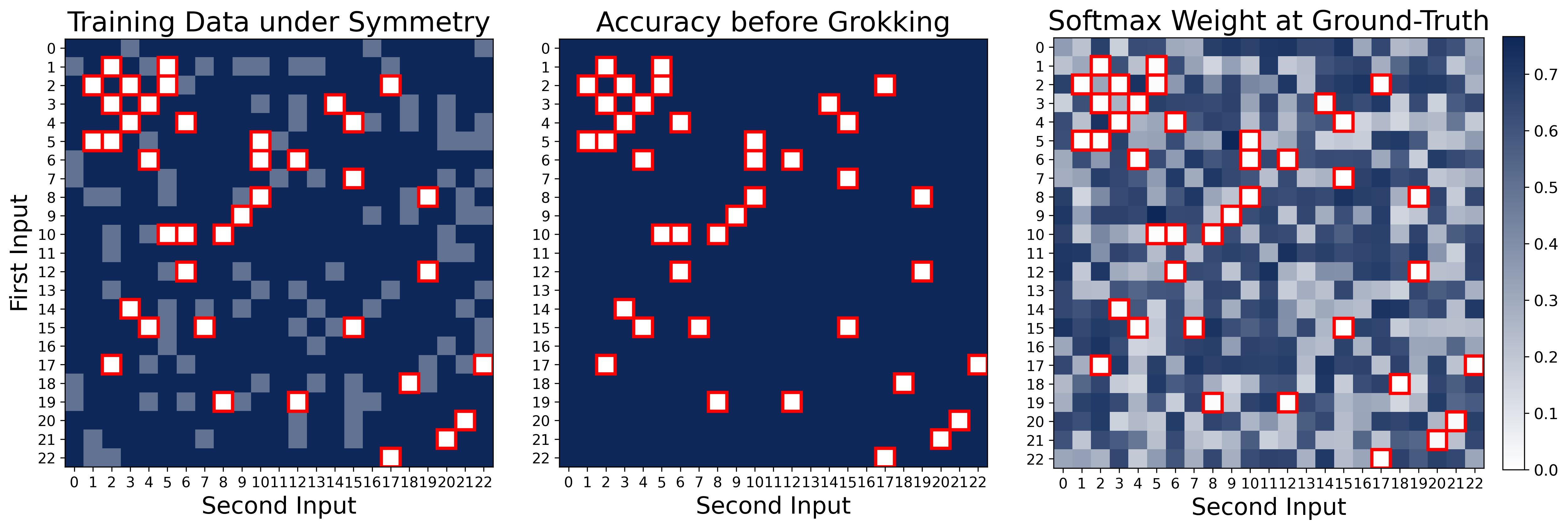 Figure 15. Accuracy heatmap at the end of the memorization stage. Each cell $(x, y)$ is colored by whether the model correctly predicts $(x+y) \bmod p$. Dark blue: training pairs, all correct (100% training accuracy). Light blue: test pairs whose symmetric partner $(y, x)$ is in the training set. These light blue cells are not in the training data, yet the model classifies them correctly “for free” because the architecture computes $\theta_m[x] + \theta_m[y]$, which is symmetric in $x$ and $y$ — so memorizing $(x,y)$ automatically gives the correct answer for $(y,x)$. White/light cells (outlined in red): truly held-out test pairs where neither $(x,y)$ nor $(y,x)$ is in the training set — completely wrong. This explains the ~70% test accuracy during Stage I: the network has memorized the training data and gets symmetric partners for free, but has not yet learned a generalizing algorithm. Generalization to the white cells requires the clean Fourier features that emerge only in Stage II.
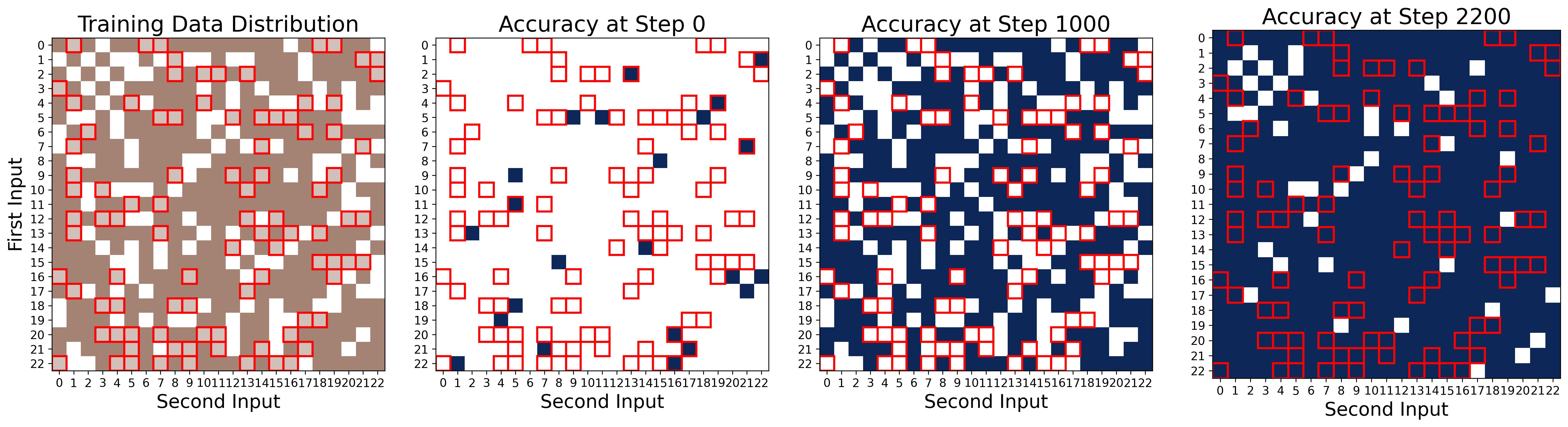 Figure 16. Common-to-rare memorization: the network learns symmetric pairs first. Four panels track accuracy during the memorization stage (Stage I). First panel (data distribution): dark brown cells are “common” (symmetric) training pairs where both $(i,j)$ and $(j,i)$ are in the training set; light brown cells (outlined in red) are “rare” (asymmetric) training pairs where only one ordering appears; white cells are held-out test data. Second panel (Step 0): at initialization, accuracy is at chance level across all data. Third panel (Step 1000): the network has memorized all common symmetric pairs (dark brown cells turn dark blue, indicating correct predictions), but accuracy on rare asymmetric pairs has been actively suppressed to zero (light brown cells remain white/incorrect). The network overwrites any initially correct random predictions on these rare examples. Fourth panel (Step 2200): the network has finally memorized the rare pairs as well, achieving 100% training accuracy. This two-phase memorization, common first, rare second, reflects the network’s architectural bias toward symmetric solutions: since $\theta_m[x] + \theta_m[y]$ is symmetric, learning $(i,j)$ automatically reinforces $(j,i)$, making symmetric pairs easier to memorize.
5.3 Stage II: Fast Generalization (Loss + Weight Decay)
After memorization, two forces compete:
- The loss gradient continues pushing magnitudes up (training loss is near-zero but not exactly zero, and the gradient remains active).
- Weight decay begins pruning non-feature frequencies, cleaning up the perturbed Fourier solution from Stage I.
The effect of weight decay is to penalize all magnitudes equally, pushing them toward zero. But the dominant (feature) frequency has much larger magnitude than the non-feature frequencies, so it can “afford” the penalty while the smaller frequencies are driven to zero. This is a sparsification effect: weight decay prunes the noisy multi-frequency representation into a clean single-frequency one.
This stage is visible in the progress measures: parameter norms keep growing (the loss gradient is still active), but frequency sparsity (measured by the inverse participation ratio, IPR) increases sharply. Test accuracy rises steeply because the cleaned-up internal representation generalizes to unseen inputs.
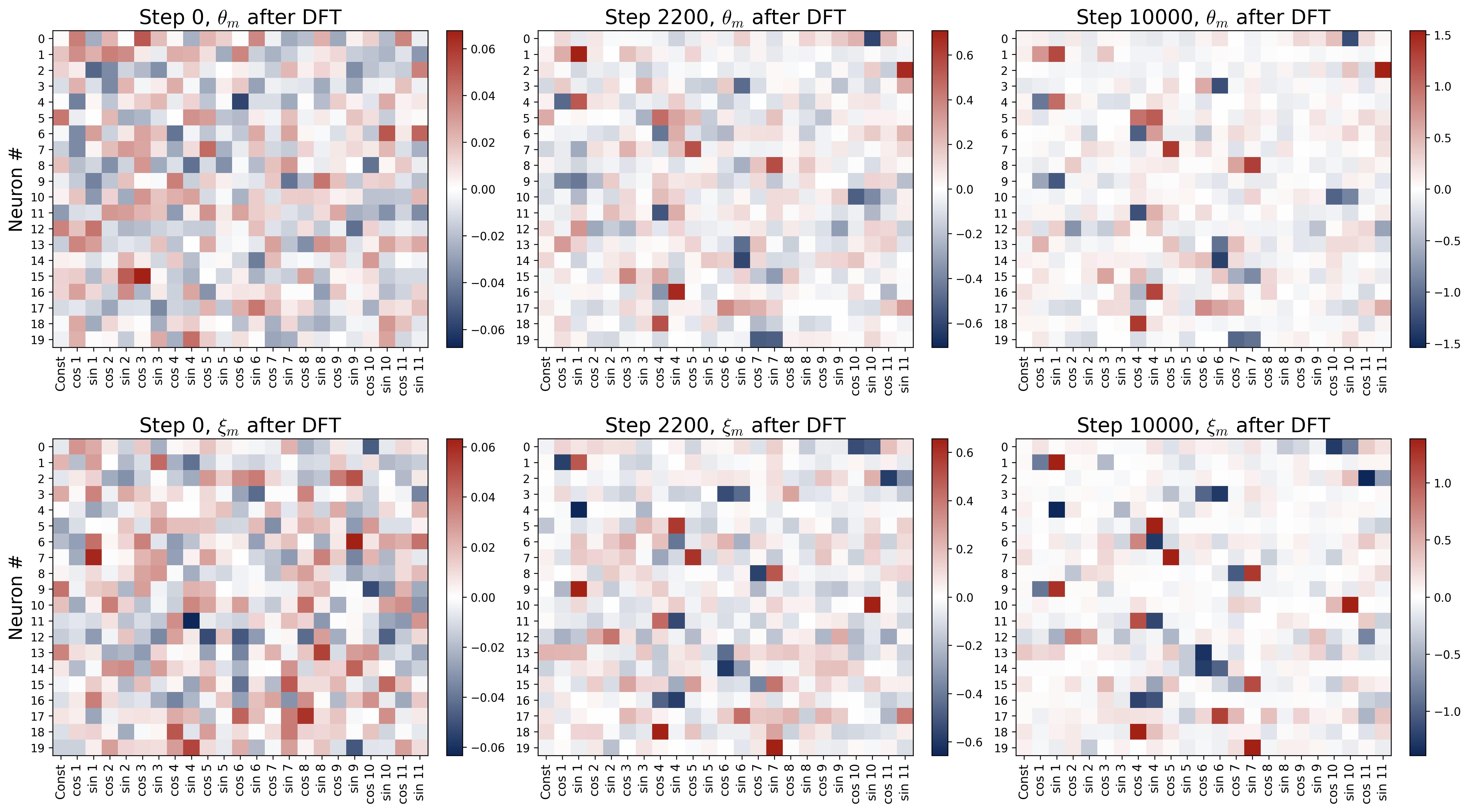 Figure 17. Weight evolution in the Fourier domain during grokking. Six panels arranged in a 2×3 grid show the DFT heatmaps of the first 20 neurons’ weights at three training snapshots ($p = 23$, train-test split). Top row: input weights $\theta_m$; bottom row: output weights $\xi_m$. Rows are neurons; columns are Fourier frequencies; color indicates DFT coefficient value. Step 0 (left): weights are diffuse across all frequencies with no discernible structure, as expected from random initialization. Step 2,200 (middle, end of memorization): a rough single-frequency pattern has started to emerge (visible as one bright cell per row), but substantial energy remains at non-feature frequencies. This is the “noisy” perturbed Fourier solution that suffices for memorization but not generalization. Step 10,000 (right, after generalization): essentially all energy resides at a single frequency per neuron, matching the clean fully-trained solution from Part I. The transition from the noisy middle panels to the clean right panels is driven by weight decay, which selectively prunes the weaker non-feature frequencies during Stages II and III.
5.4 Stage III: Slow Cleanup (Weight Decay Dominates)
Eventually, the loss gradient becomes negligible (both training and test loss approach zero). Weight decay takes over completely, slowly shrinking all parameter norms. This is visible in Figure 14(d): the IPR (frequency sparsity) continues to increase while the parameter norm decreases, confirming that weight decay is the sole active force, steadily refining the representation.
This phase is slow because there is no active driving force beyond the gentle regularizer. Weight decay alone reduces norms at rate $\partial_t \|w\| = -\lambda \|w\|$, which is exponentially slow. But it is sufficient: the feature frequencies have already been identified and their phases aligned in Stages I and II; Stage III merely fine-tunes the magnitudes.
The consequence of this cleanup is striking. Recall that during memorization (Figure 15), the white cells (truly unseen pairs where neither $(x,y)$ nor $(y,x)$ appeared in training) were completely wrong. After Stages II and III, those same pairs are now predicted correctly. This is because the cleaned-up network no longer relies on memorized associations. Instead, it implements the indicator function from Proposition 1: the majority-voting mechanism in Fourier space computes $(x+y) \bmod p$ algorithmically for any input pair, including ones never seen during training. The network has transitioned from a lookup table to a generalizing algorithm. This is grokking.
Summary of grokking. The three-stage decomposition replaces the mystery of sudden generalization with a clear narrative: the network memorizes quickly (Stage I), then weight decay cleans up the internal representation (Stage II, the “aha” moment), and finally the solution is polished (Stage III). The key insight is that generalization requires clean Fourier features, and weight decay is the force that transforms the noisy memorization solution into a clean generalizing one.
6. Conclusion
We have provided a complete reverse engineering of how a two-layer neural network learns modular addition. The results are summarized in the following table:
| Question | Answer |
|---|---|
| What does the trained network look like? | Each neuron is a cosine wave at a single frequency, with phase-locked input/output layers ($\psi = 2\phi$) and collective diversification across neurons. |
| How does it compute? | Majority voting in Fourier space: diversified neurons’ signals add coherently while noise cancels via phase symmetry, collectively approximating the indicator function on the correct sum. Softmax then sharpens this into a correct prediction. |
| How does it learn? | A lottery ticket mechanism: frequencies compete within each neuron, and the one with the best initial phase alignment wins via positive feedback (rich-get-richer dynamics). |
| Why does grokking happen? | Three stages: (I) memorization via a perturbed lottery on incomplete data, (II) fast generalization as weight decay prunes non-feature frequencies, (III) slow cleanup by weight decay alone. |
Broader Implications
Our results have several implications beyond the specific setting of modular addition:
Feature learning theory. The lottery ticket mechanism we identify, where the winning feature is determined by initial phase alignment rather than magnitude, provides a new perspective on how neural networks select features during training. The interplay between phase dynamics and magnitude dynamics may be relevant in broader settings.
The role of overparameterization. Diversification (Observation 3) requires the network width $M$ to be much larger than the number of relevant frequencies $(p-1)/2$. The surplus neurons are not wasted — they are essential for noise cancellation. This provides a concrete example of benign overparameterization, where extra parameters improve generalization by enabling collective noise cancellation.
Grokking as feature refinement. Our three-stage decomposition suggests that grokking is not a mysterious phase transition but a natural consequence of the interplay between memorization (loss minimization) and regularization (weight decay). The delayed generalization occurs because the network must first learn approximate features (which suffice for memorization) before regularization can refine them into exact features (which enable generalization).
From toy models to real networks. While modular addition is a toy task, the mathematical structures we uncover (Fourier features, phase alignment, lottery ticket competitions, and the interplay of loss and regularization during grokking) are likely to have analogs in more complex settings. Understanding these structures in a fully transparent setting is a necessary first step toward understanding them in larger, less interpretable models.
Citation
| |