Paper: In-Context Linear Regression Demystified: Training Dynamics and Mechanistic Interpretability of Multi-Head Softmax Attention
AUTHORS: Jianliang He, Xintian Pan, Siyu Chen, and Zhuoran Yang.
LINKS. ArXiv: arxiv.org/abs/2503.12734, Github: https://github.com/Y-Agent/ICL_linear .
TAKEAWAYS. We study how multi-head softmax attention models are trained to perform in-context learning on linear data. Through extensive empirical experiments and rigorous theoretical analysis, we demystify how trained multi-head attention solves in-context linear regression:
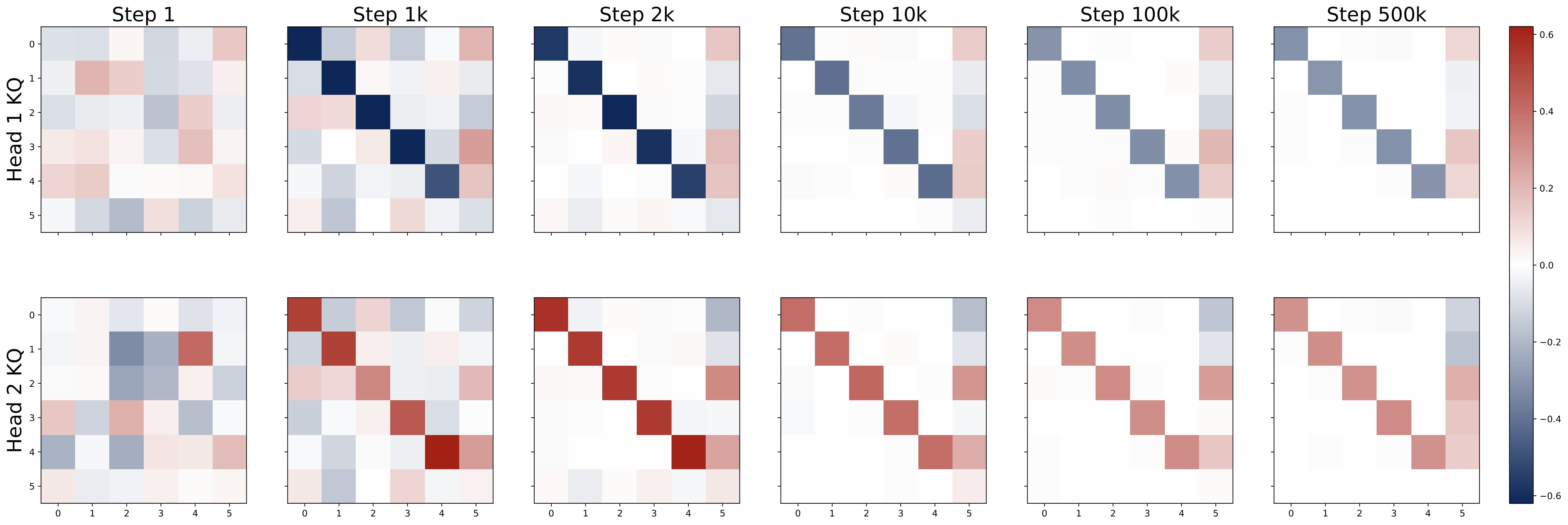
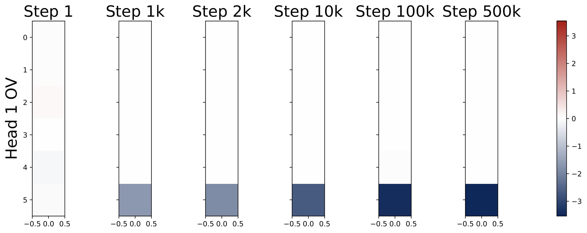
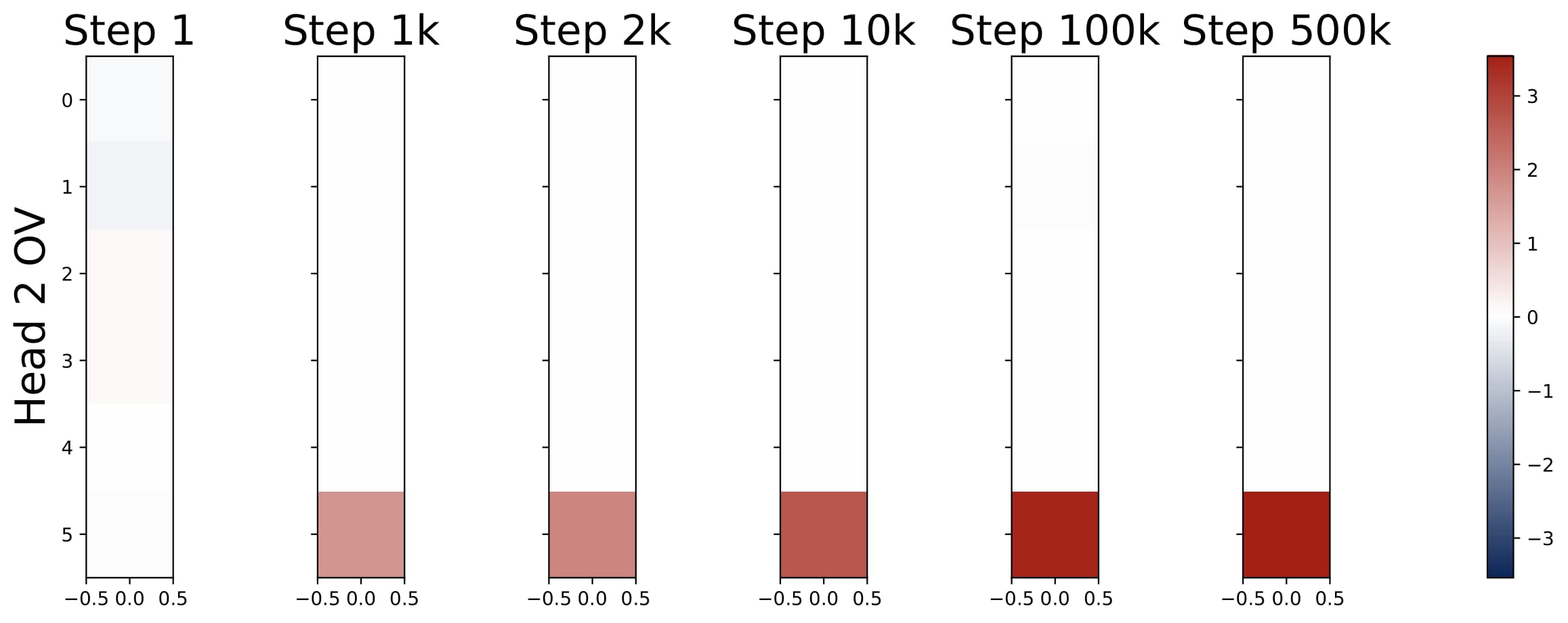
- Emergent Attention Patterns: Training reveals consistent patterns in attention matrices – diagonal and homogeneous structures in key-query (KQ) weights, and last-entry-only with zero-sum patterns in output-value (OV) weights. These patterns consistently appear from gradient-based training starting from random initialization.
- Debiased Gradient Descent: These emergent structures enable multi-head attention to implement a debiased gradient descent predictor that outperforms single-head attention and approaches Bayesian optimality.
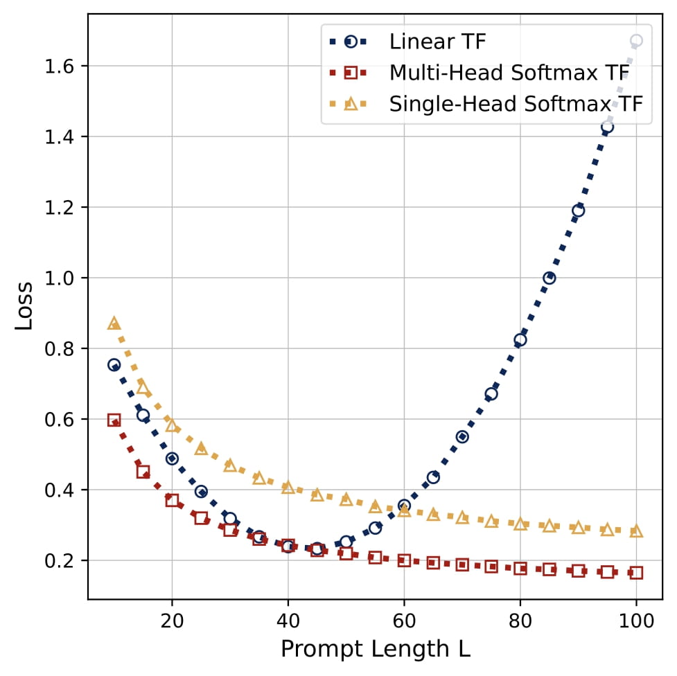
- Length Generalization: Softmax attention demonstrates superior generalization to longer sequences compared to linear transformers, maintaining effectiveness beyond training sequence lengths.
- Advanced Applications: With non-isotropic covariates, multi-head attention implements pre-conditioned gradient descent. For multi-task scenarios, a superposition phenomenon emerges at the intersection of head count and task count, efficiently resolving multi-task in-context learning.
🔍 Setups: Data Distribution and Multi-Head Attention
Data Distribution. Consider a linear regression problem where each covariate $x_\ell \in \mathbb{R}^d$ is drawn i.i.d. from $\mathsf{P}\_x$, and the regression parameter $\beta \in \mathbb{R}^d$ is drawn from $\mathsf{P}\_\beta$. Here, $\mathsf{P}\_x$ and $\mathsf{P}\_{\beta}$ are distributions over $\mathbb{R}^d$. A response $y_\ell$ is generated by $y\_\ell = \beta^\top x_\ell + \epsilon_\ell$, where $\epsilon_\ell$ is Gaussian noise. We then take a test input $x_q \sim \mathsf{P}\_x$ and embed it together with the training samples $\\{(x_\ell, y_\ell)\\}_{\ell=1}^L$ into a matrix
$$ \begin{align} Z_\mathsf{ebd}=\begin{bmatrix}Z & z_q\end{bmatrix} = \begin{bmatrix} x_1 & \dots & x_L & x_q \\\ y_1 & \dots & y_L & 0 \end{bmatrix}. \end{align} $$Here, each column of $Z_\mathsf{ebd}$ is a $(d+1)$-dimensional vector, whose first $d$ entries corresponds to the covariate and the last entry is the response. We put the query in the last column. Since we do not have the response $y_q = \beta^\top x_q + \epsilon$, we put a zero at the $(d+1, L+1)$-th entry at $Z\_\mathsf{ebd}$. Such setup is widely considered in literature (e.g., Garg et al., 2022 , Ahn et al., 2023 , Zhang et al., 2024 ).
For now, we focus mainly on the isotropic case where $\mathsf{P}\_x=\mathcal{N} (0,I_d)$ and $\mathsf{P}\_\beta=\mathcal{N}(0,I_d/d)$. Later we will also consider the non-isometric cases, i.e., $\mathsf{P}\_x=\mathcal{N}(0,\Sigma)$ for some general $\Sigma\in\mathbb{R}^{d\times d}$. Here $\mathcal{N} (\mu, \Sigma)$ is the multivariate Gaussian distribution.
In-Context Learning. In-context learning refers to a model’s ability to adapt to new tasks using only examples within its input context, without updating its parameters. In the context of regression, this means that, when a new regression task $\beta$ is generated, the model can predict $y_q$ accurately based on the data $Z_\mathsf{ebd}$. We train a one-layer transformer to solve this task.
Multi-Head Softmax Attention. A single-layer, multi-head attention model with parameters $\theta=\{O^{(h)},V^{(h)},K^{(h)},Q^{(h)}\}_{h\in[H]}\subseteq\mathbb{R}^{(d+1)\times(d+1)}$:
$$\mathrm{TF}\_\theta(Z_\mathsf{ebd})=Z_\mathsf{ebd}+\sum_{h=1}^HO^{(h)}V^{(h)}Z_\mathsf{ebd}\cdot\mathrm{smax}\circ{\rm msk}\big(Z_\mathsf{ebd}^\top K^{(h)^\top}Q^{(h)}Z_\mathsf{ebd}\big)\in\mathbb{R}^{(d+1)\times(L+1)}. $$where $\mathrm{smax}(\cdot)$ is the column-wise softmax operation, and ${\rm msk}(\cdot)$ applies a causal mask. We denote $KQ^{(h)} = K^{(h)\top}Q^{(h)}$ and $OV^{(h)} = O^{(h)}V^{(h)}$, referred to as KQ and OV circuits, which are all $(d+1)\times (d+1)$-dimensional square matrices. These matrices determine how query tokens attend to keys and how attended tokens contribute to output.
Based on the output matrix of the transformer, we extract the prediction $\hat{y}\_q$ from its $(d+1,L+1)$-th entry. That is, we let
$$ \hat{y}\_q:=\hat{y}\_q(x\_q;\{(x\_\ell,y\_\ell)\}\_{\ell\in[L]})={\rm TF}\_\theta(Z\_\mathsf{ebd})_{d+1,L+1}\in\mathbb{R}. $$Using the definition of the input data $Z_\mathsf{ebd}$ and the definitions of KQ and OV circuits, we can write $\hat y_q$ in closed form: \begin{align} \hat y_q = \sum_{h=1}^H (OV^{(h)})_{d+1} Z \cdot \mathrm{smax} \big(Z ^\top KQ^{(h)} x_q \big)\in\mathbb{R} \end{align} Here, $(OV^{(h)})_{d+1}$ is the last row of $OV^{(h)}$.
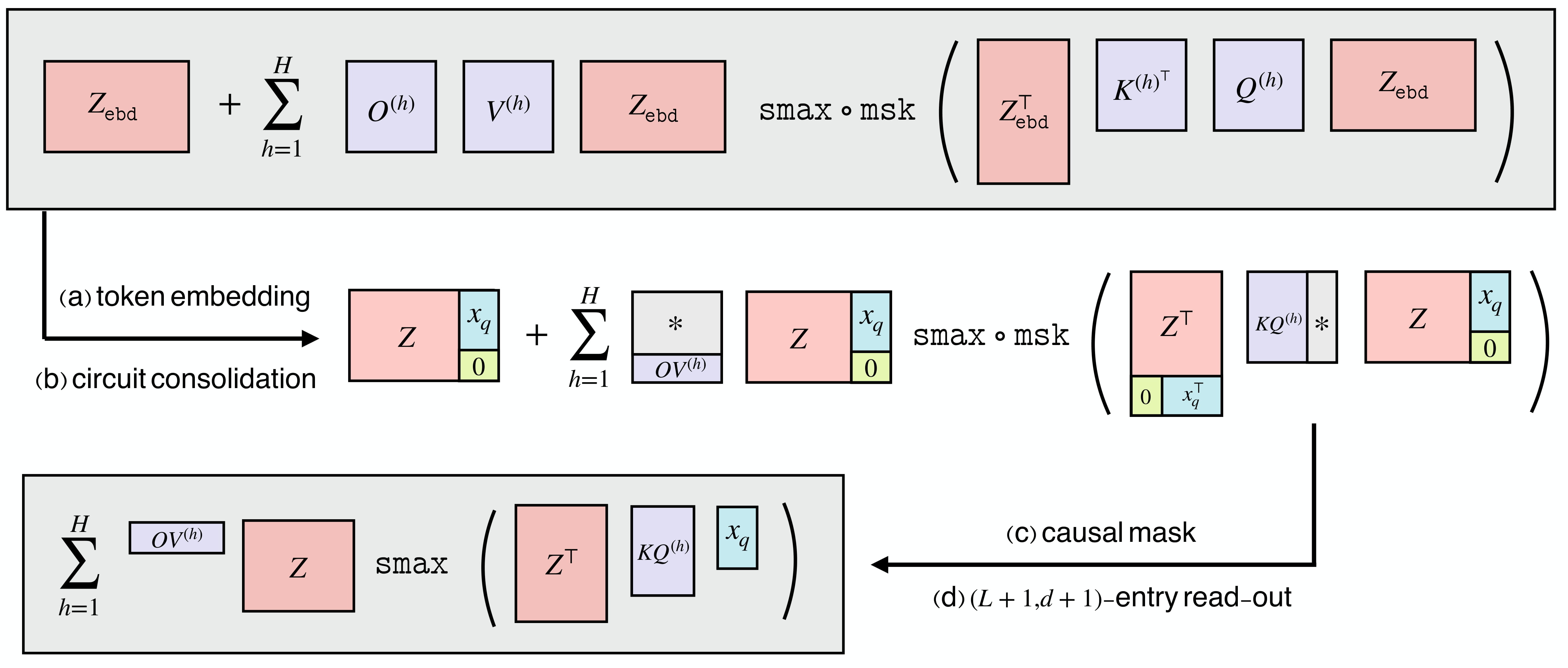
Interpretation of the Transformer Model. To get the output, we use $Q^{(h)}x_q$ as the query, which attends to the keys $\\{ K^{(h)} x\_{\ell}\\}\_{\ell\in[:L]}$. After applying softmax, we get a probability distribution over $[L] = \\{1, \ldots, L\\}$. This probability is used to aggregate the corresponding values $\\{ V^{(h)} x\_{\ell}\\}\_{\ell\in[:L]}$ to get the output. We use the term circuits to refer to the KQ and OV matrices, i.e., $KQ^{(h)}$ and $OV^{(h)}$, which are the key components of the attention mechanism. This follows from the same terminology as in Olsson et al. (2022) .
Training Setup. To investigate how the model learns to solve linear regression in context, we train by minimizing the mean-squared error (MSE). The population loss follows
$$ \mathcal{L}(\theta)=\mathcal{E}(\hat{y}\_q)=\mathbb{E}[(y_q-\hat{y}\_q)^2]=\mathbb{E}[(y_q-{\rm TF}\_\theta(Z\_\mathsf{ebd})\_{d+1,L+1})^2]. $$Here, the expectation is over the random draw of $\beta \sim \mathsf{P}\_\beta$ and the samples $\\{(x_\ell, y_\ell)\\}\_{\ell\in[L]}$ drawn i.i.d. from $\mathsf{P}\_x \otimes \mathsf{P}\_{y|x}(\cdot;\beta)$. Training proceeds via mini-batch stochastic gradient methods: at iteration $t$, we sample $n_{\text{batch}}$ regression parameters from $\mathsf{P}\_\beta$ and generate an equal number of embedded sequences $Z_{\text{ebd}}$. We then approximate $\nabla \mathcal{L}(\theta_t)$ and update $\theta_t$ as
$$ \theta_{t+1} \;\leftarrow\; \mathsf{UpdateMethod}\bigl(\theta_t,\;\widehat{\nabla}\mathcal{L}(\theta_t)\bigr), $$where the update method can be gradient descent, Adam, or another optimizer.
📚 Empirical Insights: Emerged Patterns and Dynamics
We performed experiments to understand how multi-head softmax attention learns linear regression tasks through in-context learning (ICL). We consider the setting with isotropic covariates, i.e., $\mathsf{P}_x = \mathcal{N} (0,I_d)$ and vary $H$ (the number of heads) in our experiments. All experiments use a data setup with $L = 40$, $d = 5$, and noise variance $\sigma^2 = 0.1$. Models are trained using Adam with learning rate $\eta = 10^{-3}$, batch size $256$ for $5 \times 10^5$ steps, starting from PyTorch’s default random initialization. We remark that variations in optimization algorithm, hyperparameters, or the data-generating process do not significantly affect the results.
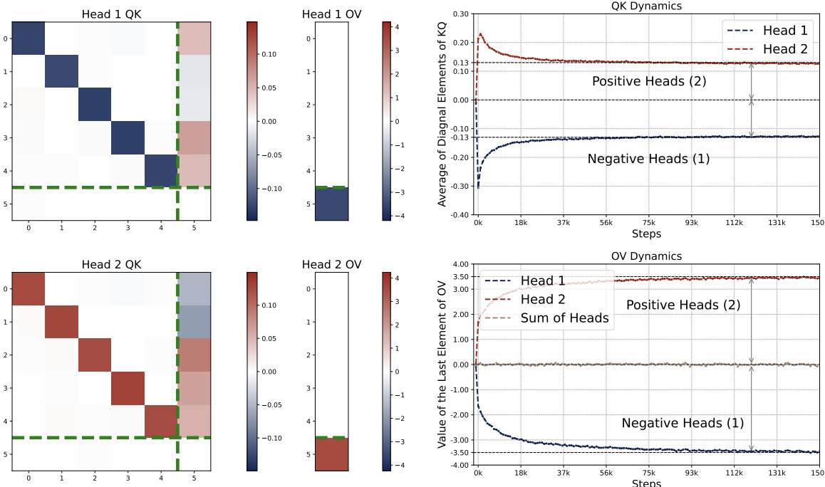
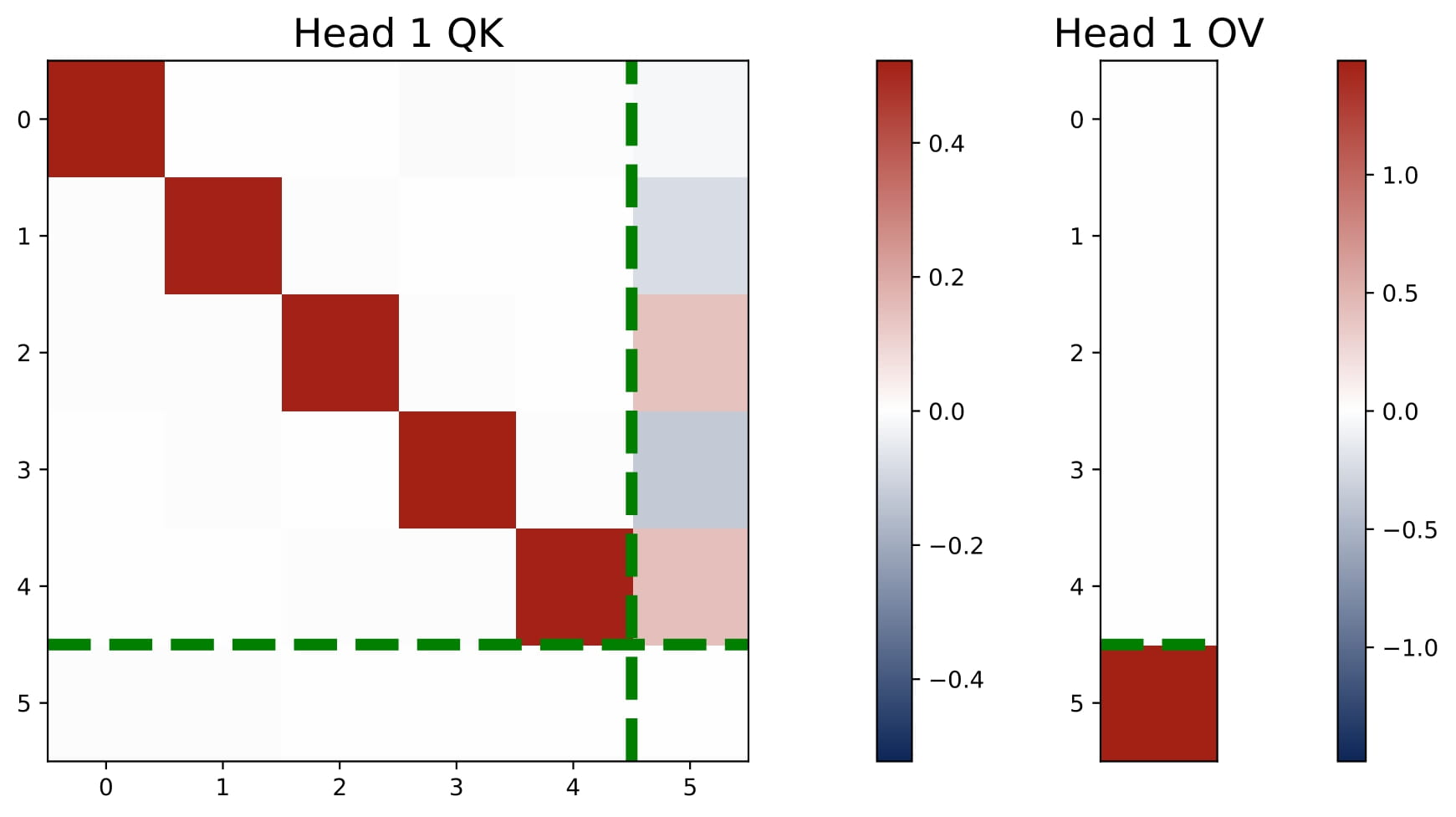
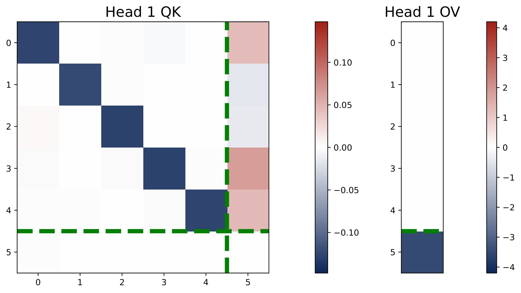
💎 Key Finding 1: Global KQ/OV Patterns.
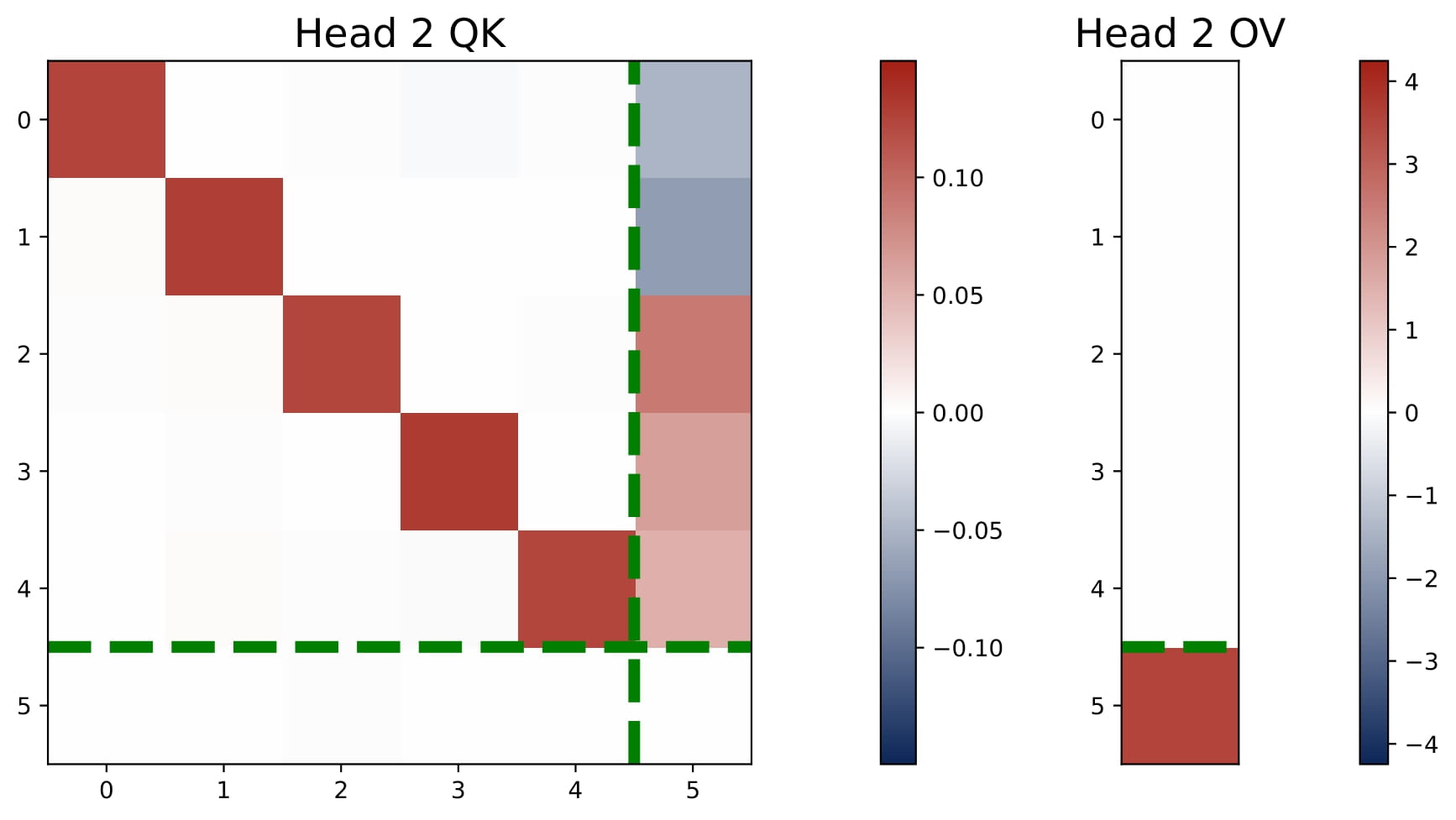
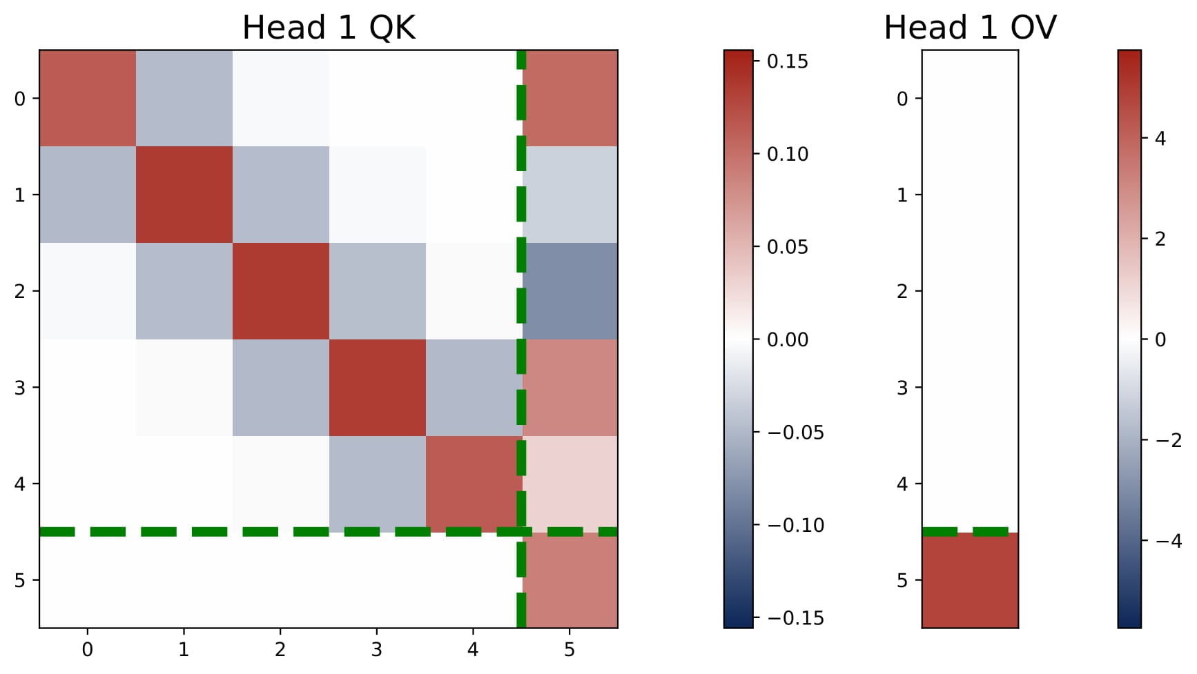
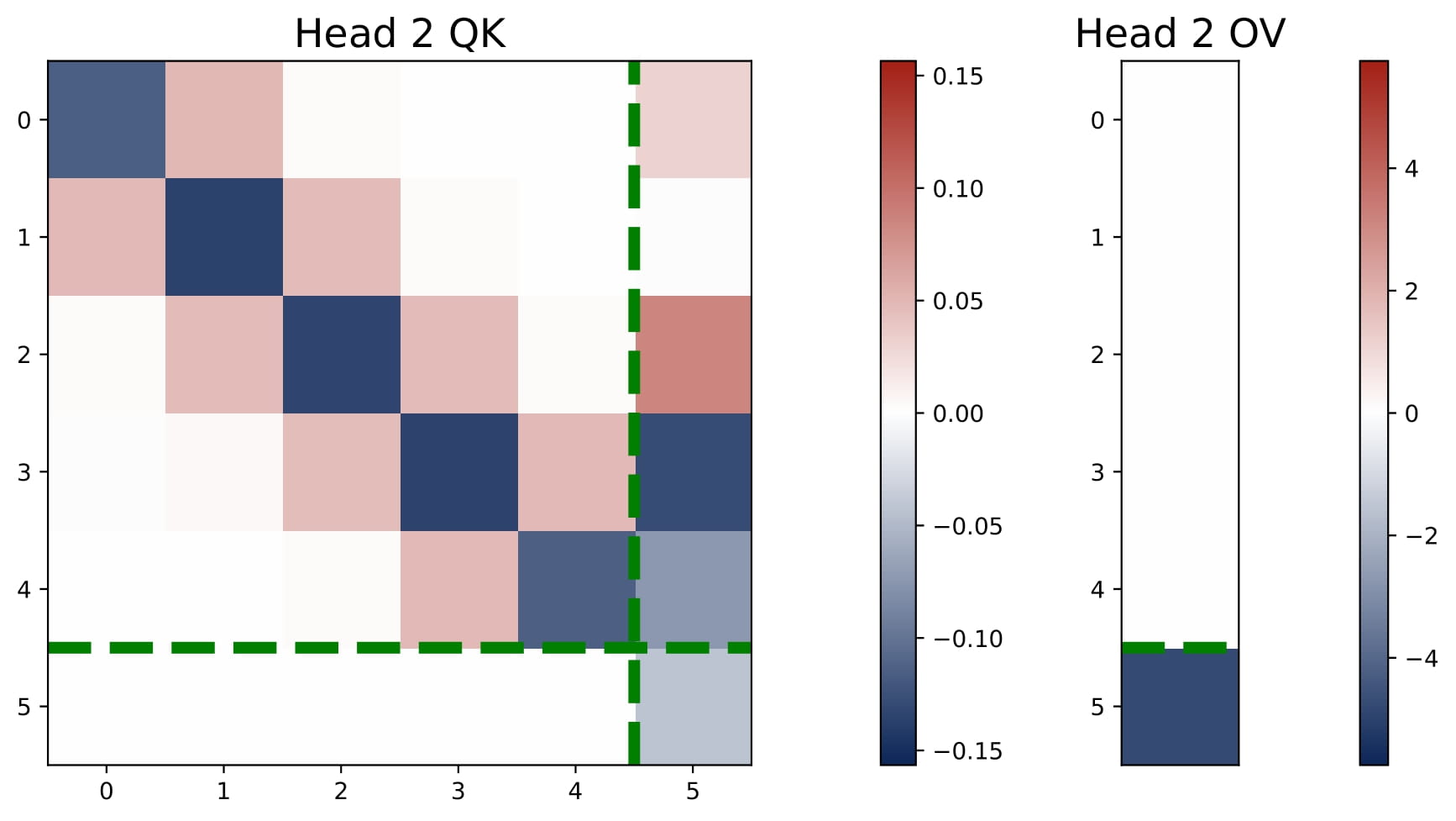
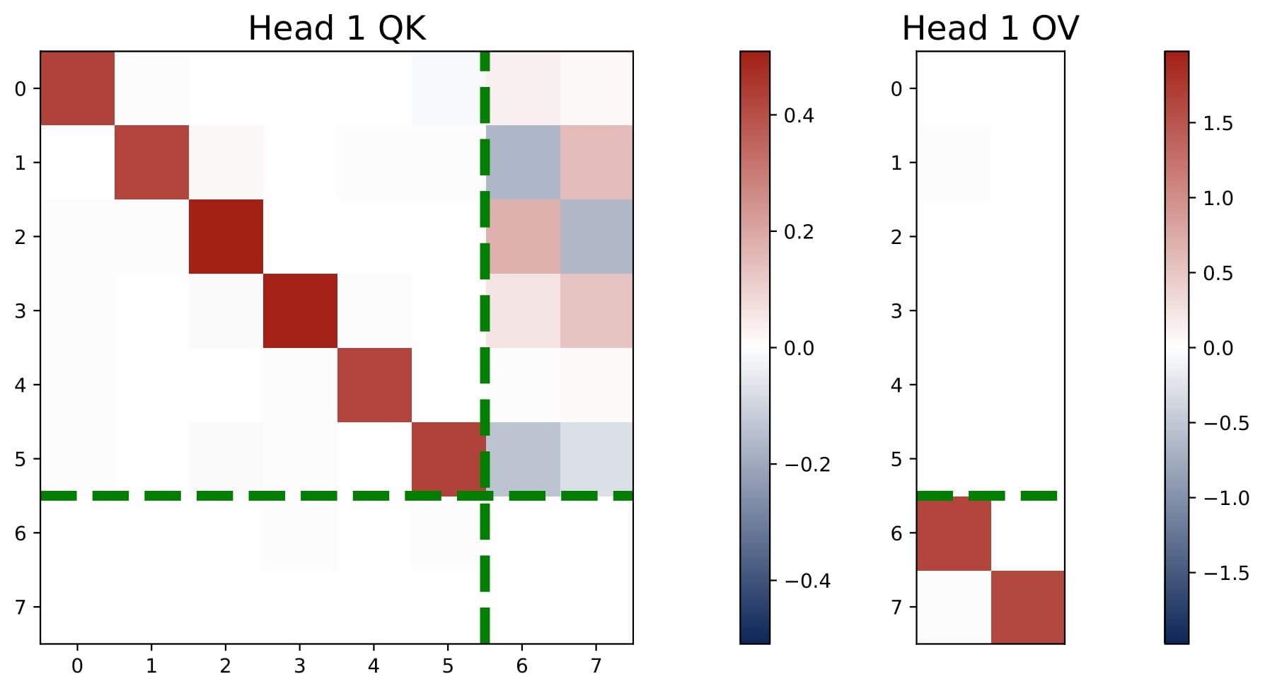
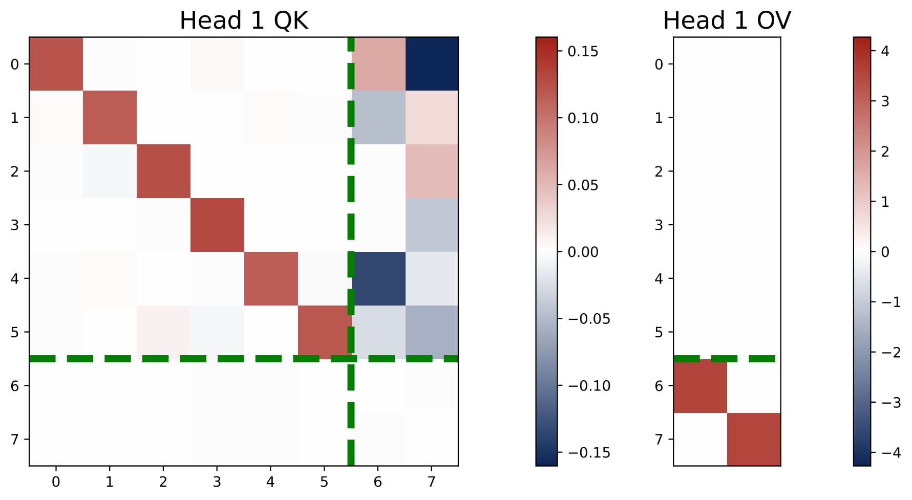
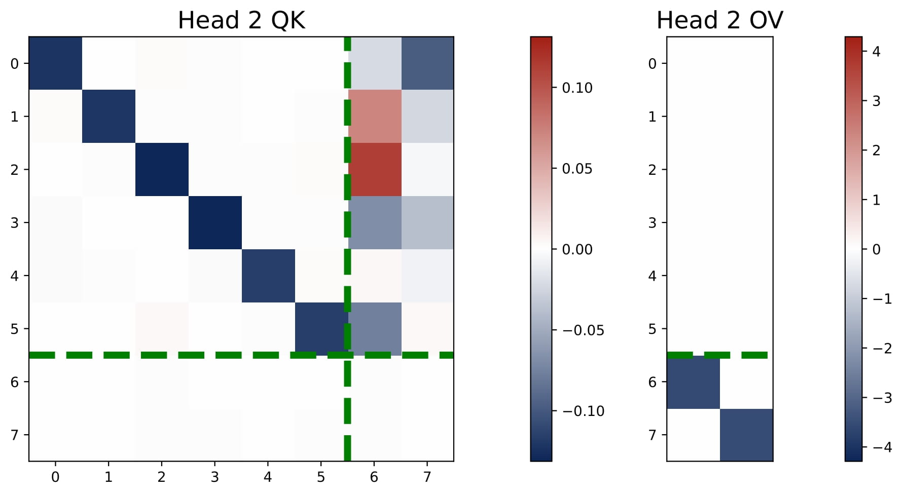
For any number of heads with $H \geq 1$, in the trained one-layer multi-head attention model, the KQ and OV circuits take the following form: for all $h\in[H]$, we have
$$ KQ^{(h)} = \begin{bmatrix} \omega^{(h)} \cdot I_d & \ast \\\ \mathbf{0}_d^\top & \ast \end{bmatrix} \in \mathbb{R}^{(d+1)\times(d+1)}, \quad OV^{(h)} = \begin{bmatrix} \ast & \ast \\\ \mathbf{0}_d^\top & \mu^{(h)} \end{bmatrix} \in \mathbb{R}^{(d+1)\times(d+1)}. $$Here $\omega^{(h)}$ and $\mu^{(h)}$ are two numbers. That is, the top $d$-by-$d$ submtraix of each KQ circuit is a diagonal matrix (in the case $\mathsf{P}_x = \mathcal{N} (0,I_d)$, the diagonal matrix is proportional to an identity matrix), and the rest of the entries are ineffective. The bottem-right entry of each OV circuit is the only effective entry, and it is denoted by $\mu^{(h)}$.
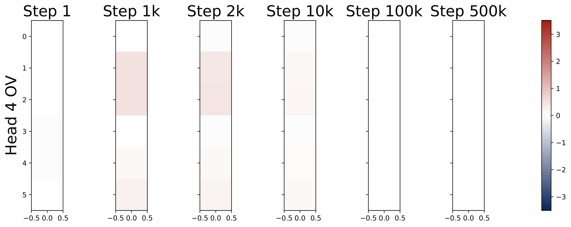
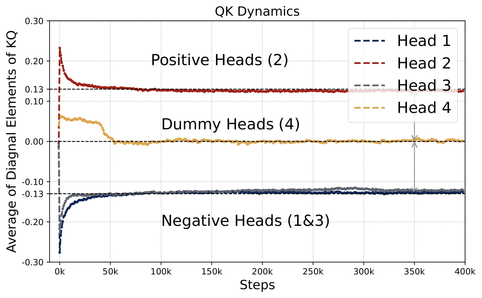
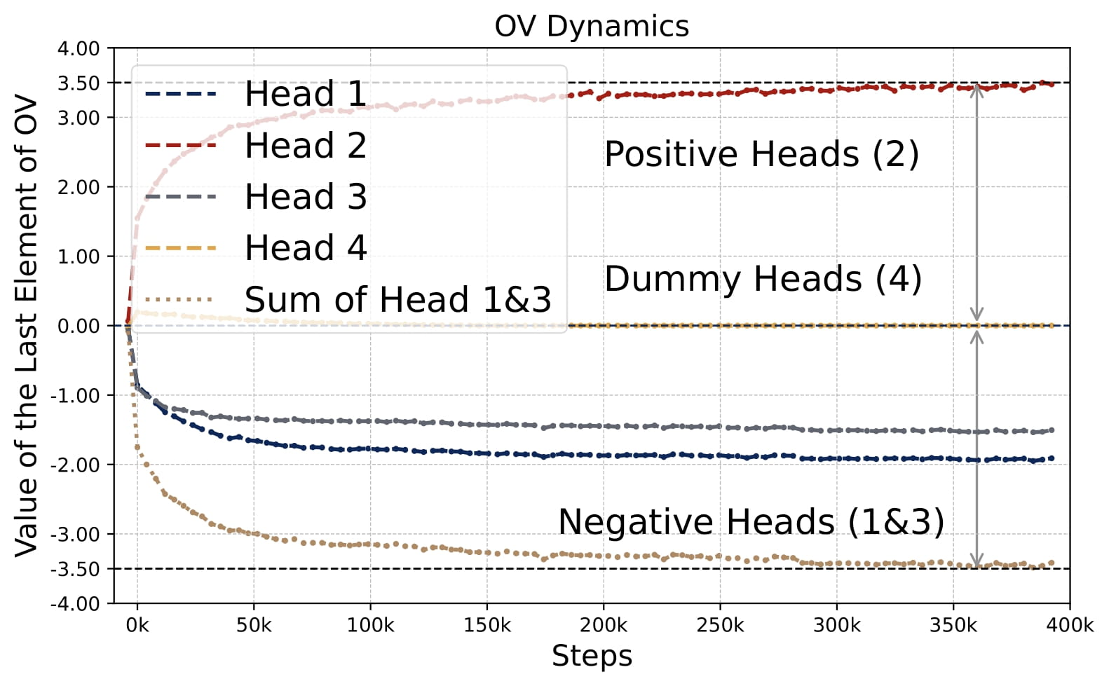
Moreover, the KQ and OV circuits share the same signs within each head, i.e., $\mathrm{sign}(\omega^{(h)}) = \mathrm{sign}(\mu^{(h)})$. We refer to this property as sign-matching. Thus, each head can be categorized into either a positive or negative head depending on the sign of $\omega^{(h)}$, defined by $\mathcal{H}\_+=\\{h:\omega^{(h) }> 0\\}$ and $\mathcal{H}\_-=\\{h:\omega^{(h)}< 0\\}$. In some cases, dummy heads may emerge, where $\omega^{(h)}\approx0$ and $\mu^{(h)}\approx0$. Remarkably, these patterns develop early in training and remain consistent throughout the optimization process.
These global patterns appear in all attention models with $H \geq 1$.
The global patterns of KQ and OV circuits show that the weight matrices of the learned transformer essentially are governed by $2H$ numbers $\\{ \omega^{(h)}\\}\_{h\in[H]}$ and $\\{\mu^{(h)} \\}\_{h\in[H]}$, denoted by $\mu = (\mu^{(1)}, \dots, \mu^{(H)})^\top$ and $\omega = (\omega^{(1)}, \dots, \omega^{(H)})^\top$. Under such a structure, the transformer predictor takes the form:
\begin{align} \hat{y}_q &=\sum_{h=1}^H\mu^{(h)}\cdot\bigl\langle y,{\rm smax}(\omega^{(h)}\cdot Xx_q)\bigr\rangle=\sum_{h=1}^H\mu^{(h)}\cdot\sum_{\ell=1}^L\frac{y_\ell\cdot\exp(\omega^{(h)}\cdot x_\ell^\top x_q)}{\sum_{\ell=1}^L\exp(\omega^{(h)}\cdot x_\ell^\top x_q)}\in\mathbb{R}. \end{align}
Thus, each head acts as a separate kernel regressor, and thus the attention model can be interpreted as the sum of kernel regressors.
💎 Key Finding 2: Learned Values of $(\omega,\mu)$.
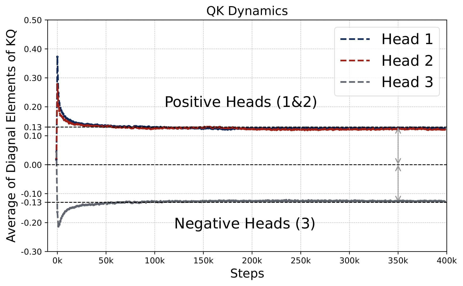
Note that the model is effectively governed by parameters $(\omega,\mu) \in \mathbb{R}^{2H}$. For each head $h$, $\omega^{(h)}$ scales its key-query block and $\mu^{(h)}$ sets the output weight in the OV circuit. Two main observations emerge when $H \ge 2$ (see Figure 2.2):
- Homogeneous KQ Scaling. The scaling of the top-left diagonal submatrix of each $KQ^{(h)}$ of non-dummy heads is nearly identical across all positive and negative heads, $\omega^{(h)}$, meaning $\lvert \omega^{(h)} \rvert \approx \gamma$ for all $h\in\mathcal{H}\_+\cup\mathcal{H}\_-$.
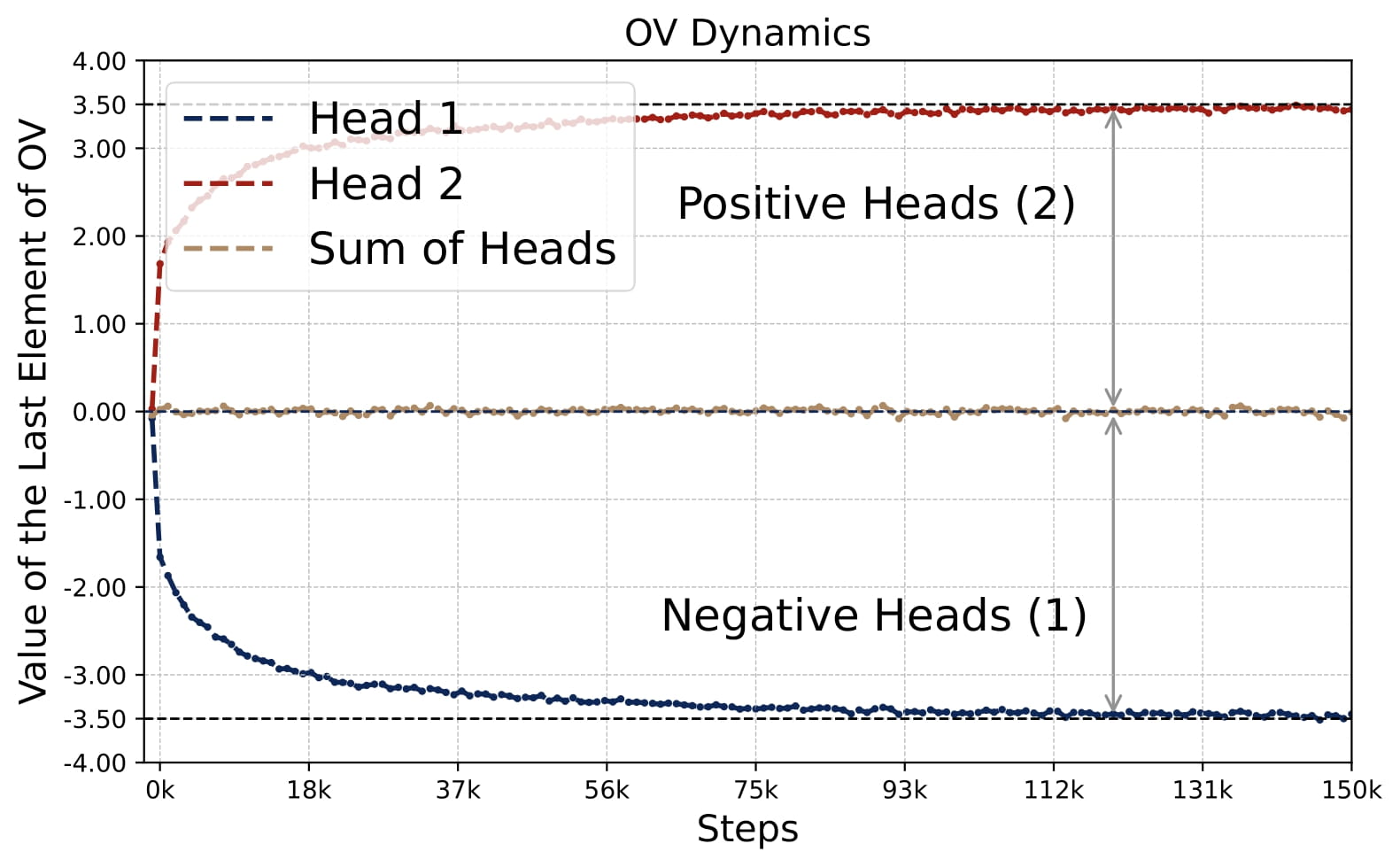
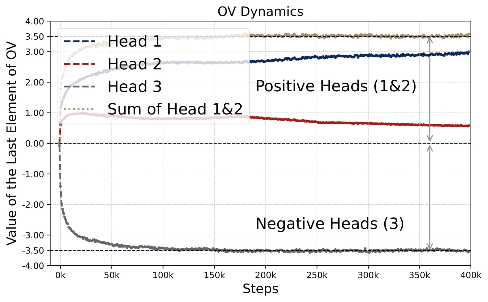
- Zero-Sum OV. The sum of all $\mu^{(h)}$ across heads is approximately zero, implying positive and negative heads balance each other out $\sum\_{h\in\mathcal{H}\_{+}} \mu^{(h)} \approx -\sum\_{h\in\mathcal{H}\_{-}} \mu^{(h)}$.
Thus, multi-head attention models typically have at least one positive head and one negative head, unlike the single-head case which is always purely positive or negative (see Figure 2.1). When $H>2$, similar patterns persist, although dummy heads may emerge. See Figure 2.8.
💎 Key Finding 3: Multi-Head Outperforms Single-Head, Approximates Gradient Descent
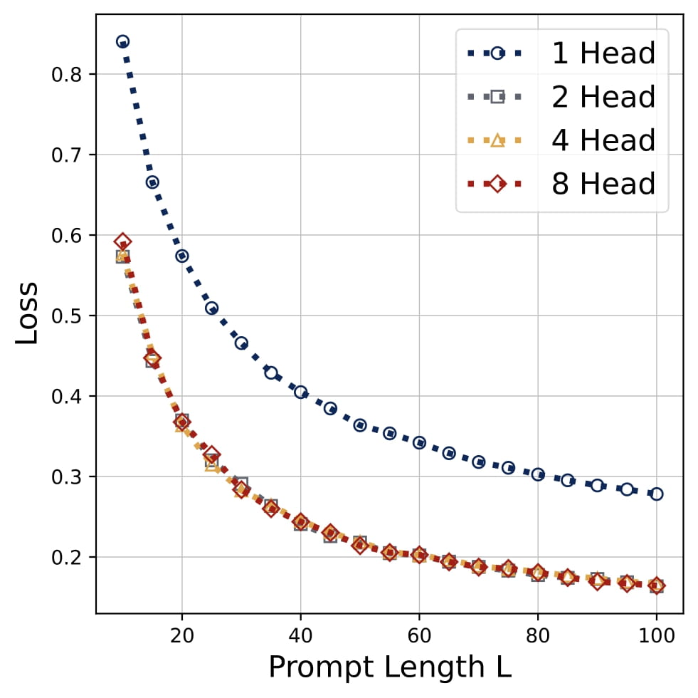
- Performance: In terms of the ICL prediction error, the two-head attention model outperforms single-head model. Surprisingly, all multi-head configurations $H=2, 3, 4, \dots$ attains nearly the same performance, indicating that the multi-head attention models all learn the same predictor when $H \geq 2$.
Comparison to Gradient Descent: The learned multi-head predictors closely match the vanilla one-step gradient descent (GD) solution on $\\{(x_\ell,y_\ell)\\}\_{\ell\in[L]}$. Empirically, the error curves of multi-head models track GD and outperform single-head attention. They also generalize to longer sequences $L$ than those seen in training. In fact, the attention model learns to implement a debiased GD:
$$ \eta /L \cdot \bar x_{\ell}^\top x_q \cdot y_{\ell}, \qquad \textrm{where} \quad\bar x_\ell=x_\ell-{L}^{-1}\cdot \sum_{\ell=1}^Lx_\ell. $$Here the learning rate $\eta$ is determined by the learned values of the KQ and OV circuits, and is close to one when $L$ is large. Furthermore, since $\mathbb{E}[x_\ell]=0$, when $L$ is large, the debiased GD predictoir coincides with the vanilla GD predictor $\eta /L \cdot x_{\ell}^\top x_q \cdot y_{\ell}$
Single-Head Attention vs. Multi-Head Attention The multi-head attention models learn a different predictor from the single-head attention model. In terms of the values of the parameters, As proven in Chen et al. (2024a) , in a single-head attention model, we have $\omega^{(1)} = 1/\sqrt{d}$ and $\mu^{(1)} = \Theta(\sqrt{d})$. In the multi-head attention models, the magnitude of the KQ circuits, $|\omega^{(h)}|$, is much smaller than $1/\sqrt{d}$. Qualitatively speaking, single-head attention learns a Nataraya-Watson (nonparametric) predictor, whereas multi-head attention learns a GD (parametric) predictor.
Near-Bayes Performance: While the optimally tuned ridge estimator remains the theoretical Bayes-optimal for isotropic Gaussian data, multi-head attention’s mean-squared error nearly achieves Bayesian optimality up to a proportional factor.
💎 Key Finding 4: Consistent Training Dynamics
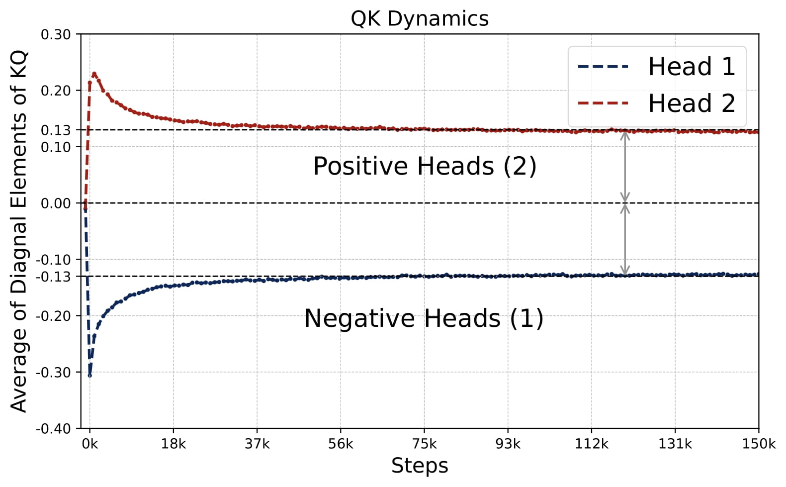
- Emergence of Patterns: Despite random initializations, the parameter evolution follows a highly consistent trajectory throughout training. As shown in Figure 2.5, the attention model quickly develops the pattern identified in Key Finding 1, during the early stages of training. The attention model continues to optimize the loss function with this pattern preserved throughout the training process.
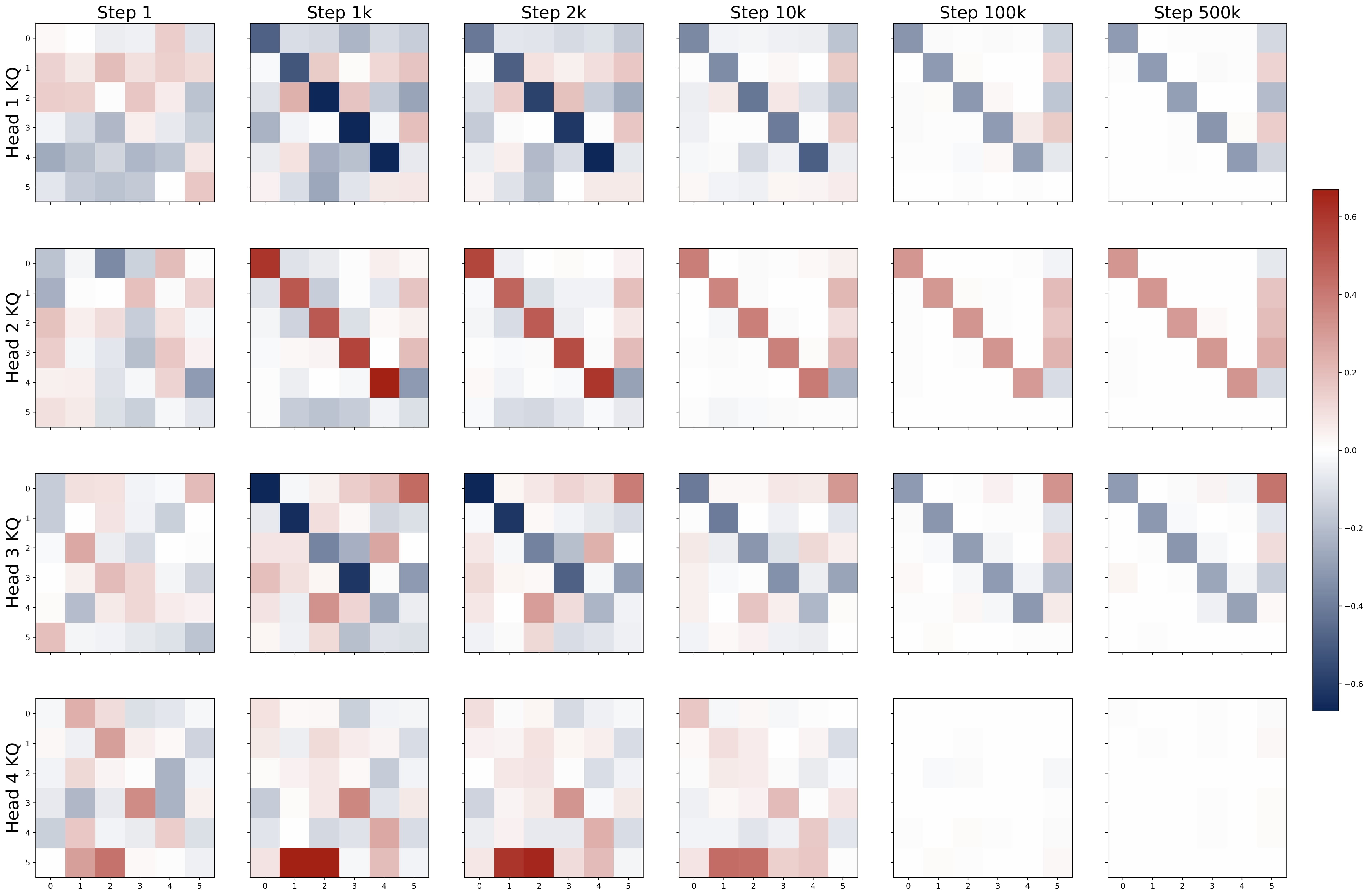
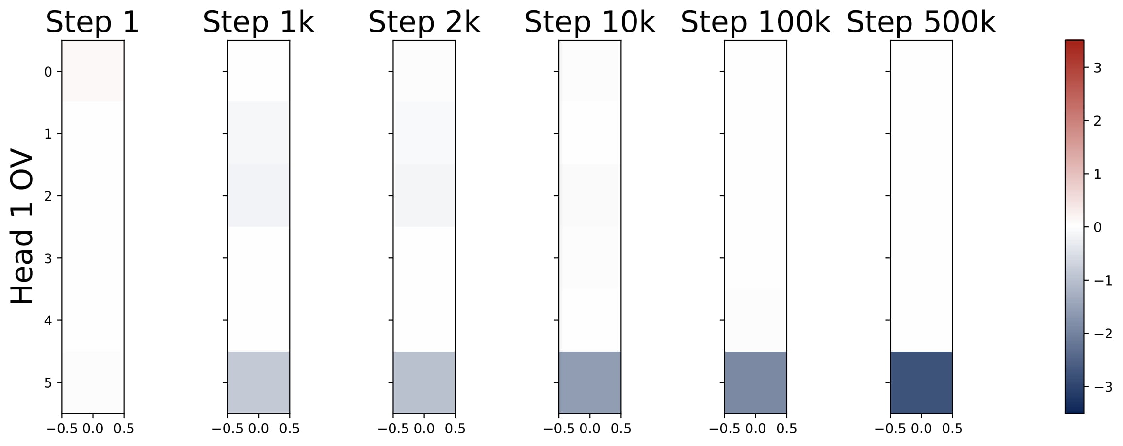
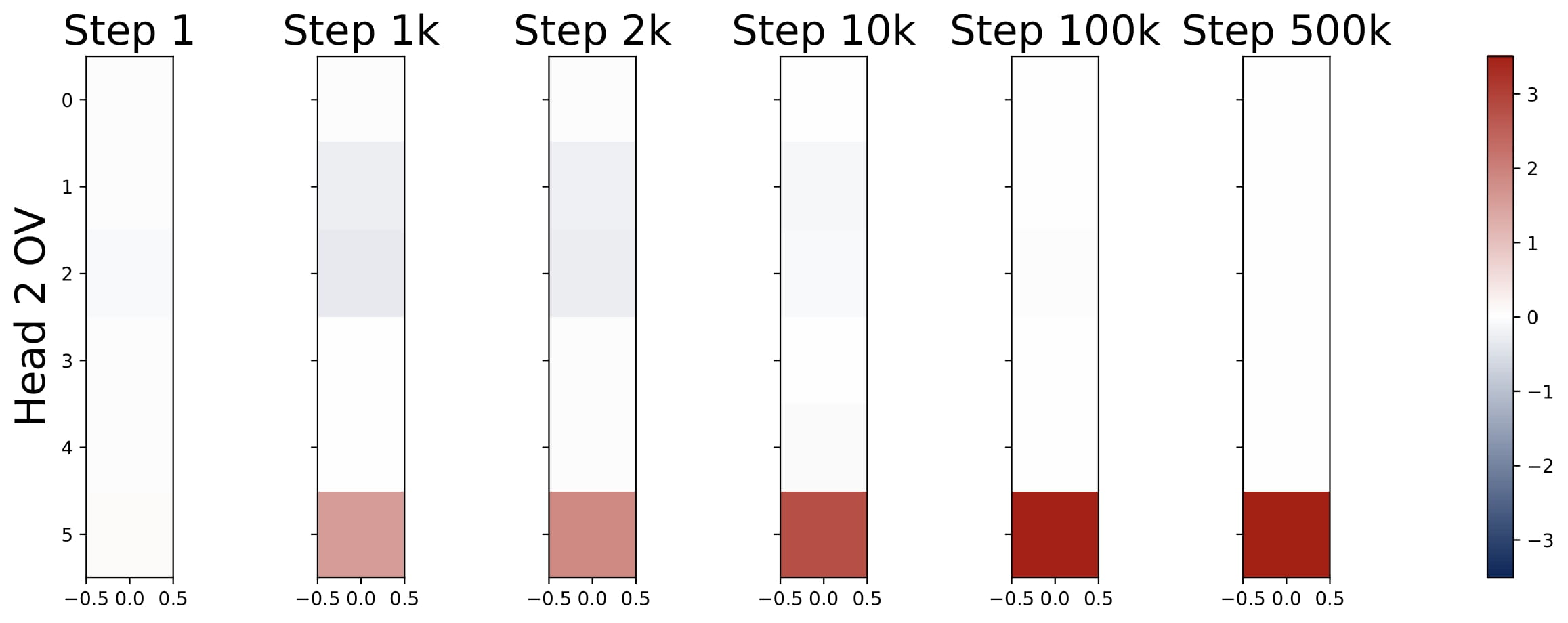
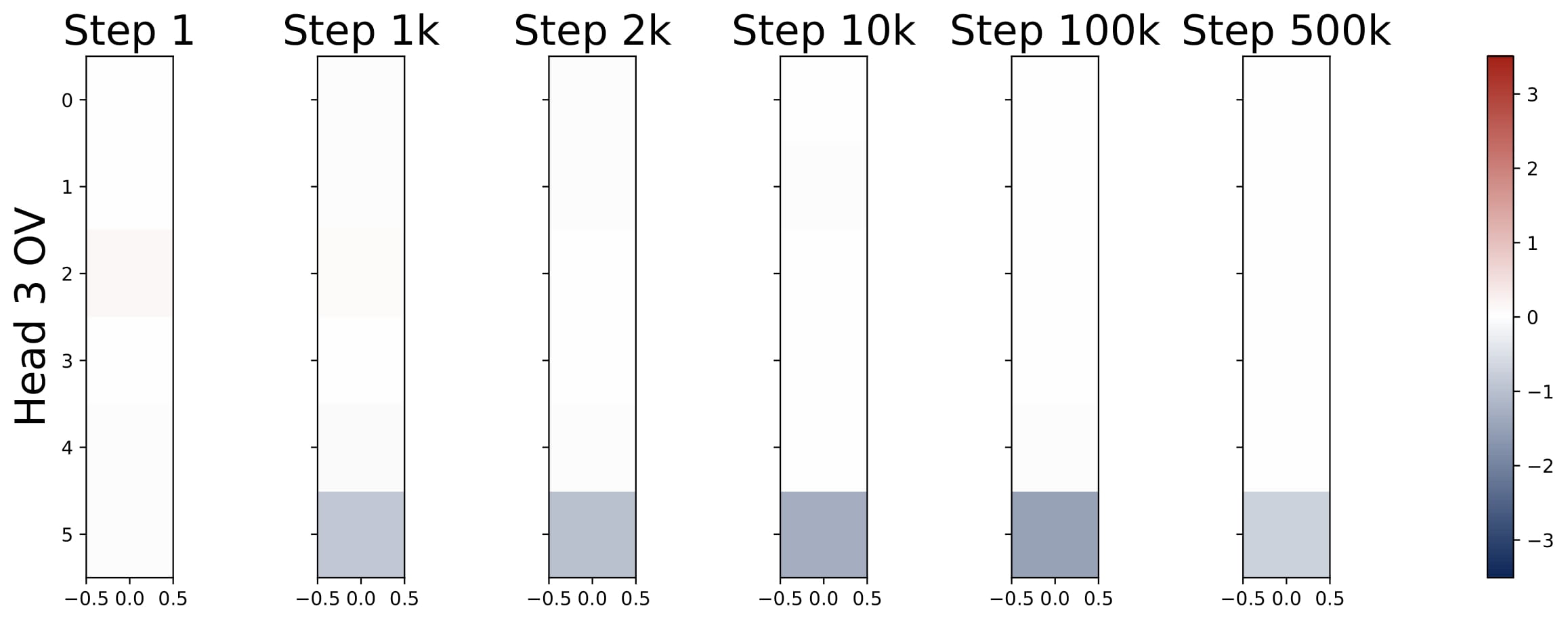
- Parameter Evolution: The training dynamics of the KQ circuits are not monotonic. The magnitudes of $\omega^{(h)}$’s first increase and then decrease to stabilize. Whereas the magnitude of OV circuits, i.e., $\sum_{h\in \mathcal{H}_+} \mu^{(h)}$, increases steadily throughout training. More importantly, for different model sizes, as long as $H \geq 2$, the limiting values are approximately the same! (0.13 for KQ and 3.5 for OV.)
🧭 Extensions
💎 Non-Isotropic Covariates
When covariates are drawn from a centered Gaussian with a general covariance matrix $\Sigma$, softmax attention still learns a sum of two kernel regressors —— but the KQ blocks need not be diagonal. Here, we consider the two-head model for illustration. Concretely:
- Persistent OV Patterns: The last-entry-only structure in the OV circuits continues to emerge, splitting heads into a positive and a negative group.
Here $\mu$ is a positive scalar.
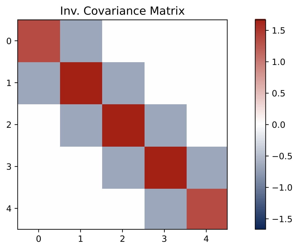
- KQ as a Preconditioner: Instead of a diagonal as in the isotropic case, the KQ block becomes a dense matrix with a small magnitude, denoted by $\gamma \cdot \Omega$, where $\gamma$ is a small and positive scalar and $\Omega$ is close to $\Sigma^{-1}$. This matrix effectively preconditions the regression problem by replacing $x_q^\top x_\ell$ with $x_q^\top \Omega\,x_\ell$.
- Approximate Preconditioned GD: For small $\gamma$, the learned transformer approximates a debiased preconditioned gradient descent predictor
Empirically, $\Omega$ often appears close to the inverse covariance matrix, i.e., $\Omega\approx\Sigma^{-1}$, especially when $L$ is large. This coincides with the estimator learned by linear transformers.
In short, multi-head softmax attention naturally learns to incorporate covariance information in the KQ circuit, yielding a preconditioned GD predictor that adapts to non-isotropic data.
💎 In-Context Multi-Task Regression
We also consider multi-task regression, where each task uses a different subset $\mathcal{S}\_n\subseteq [d]$ of features. The transformer is now trained to predict a vector $y_q\in\mathbb{R}^N$ given $L$ demonstrations $\\{(x_\ell, y_\ell)\\}_{\ell\in[L]}$. The setup is formalized as follows.
In-Context Multi-Task Regression. Given $d\in\mathbb{Z}^+$, we assume the covariate $x\in\mathbb{R}^d$ is independently sampled from $\mathsf{P}\_x$, and let $\beta\in\mathbb{R}^{d}$ be a fixed signal parameter. Let $N\in\mathbb{Z}^+$ denote the number of tasks. For each task $n\in [N]$, let $\mathcal{S}\_n\subseteq[d]$ denote a nonempty set of indices for task $n\in[N]$. Let $\beta\_{\mathcal{S}_n}$ and $x\_{\mathcal{S}_n}$ denote the subvectors of $\beta$ and $x$ indexed by $\mathcal{S}_n$. We define the response vector $y=[y_1,\dots,y_N]^\top\in\mathbb{R}^N$ by letting $y_n=\beta\_{\mathcal{S}_n}^\top x\_{\mathcal{S}_n}+\epsilon_n$ for all $n \in [N]$, where $\epsilon_n\overset{\rm i.i.d.}{\sim}\mathcal{N}(0,\sigma^2)$.
In the ICL setting, we assume that the signal set $\\{\mathcal{S}\_n\\}\_{n\in[N]}$ is fixed but unknown. To perform ICL, we first generate $\beta \sim \mathsf{P}\_\beta$ and then generate $L$ demonstration examples $\\{ (x\_{\ell}, y\_{\ell}) \\}\_{\ell\in[L]}$ where $x\_\ell\overset{\rm i.i.d.}{\sim}\mathsf{P}\_x$ and $y_\ell$ is generated by the linear model with parameter $\beta$. Moreover, we generate another covariate $x_q \sim \mathsf{P}\_x$ and the goal is to predict the response $y_q\in\mathbb{R}^N$ for the query $x_q$.
Experimental Setups. We let $\\{(x_\ell, y_\ell)\\}\_{\ell \in [L]}$ denote the ICL examples, where $x\_\ell \in \mathbb{R}^d$ and $y_\ell \in \mathbb{R}^N$. We consider the isotropic case with $\mathsf{P}\_x = \mathcal{N}(0, I_d)$ and $\mathsf{P}\_\beta = \mathcal{N}(0, I_d / d)$. Moreover, in our experiment, we focus on the two-task case with $N=2$, $d=6$, $L=40$, $\sigma^2=0.1$. Moreover, we set $\mathcal{S}_1=\\{1, 2, 3, 4\\}$ and $\mathcal{S}\_2=\\{3, 4, 5, 6\\}$, i.e., the features of the tasks have overlap $\\{ 3, 4\\}$. We train multi-head attention models with $H \in\\{1,2,3,4\\}$, which suffices to represent all potential cases.
To simplify the notation, we let $\mathcal{S}^{\ast}=\mathcal{S}\_1\cap\mathcal{S}\_2 = \\{3,4\\}$ and $\mathcal{S}^c=[d]\backslash\mathcal{S}^{*} = \\{ 1,2, 5,6\\}$. Besides, for each $n \in [N]$, we let $y\_{\ell, n}$ denote the $n$-th entry of the response vector $y\_\ell$. For any subset $\mathcal{S}\subseteq [d]$, we let $x\_{\ell, \mathcal{S}}$ denote the subvector of $x\_\ell$ with indices in $\mathcal{S}$.
Our findings.
Global Pattern. Despite the output dimension now being $d+N$, the learned model maintains a similar global patter as in single-task setting (see Figure 3.2 below).
$$ KQ^{(h)} = \begin{bmatrix} KQ^{(h)}\_{11} & \ast \\\ KQ^{(h)}\_{21} & \ast \end{bmatrix} \in \mathbb{R}^{(d+N)\times(d+N)}, \quad OV^{(h)}= \begin{bmatrix} \ast & \ast \\\ OV^{(h)}\_{21} & OV^{(h)}\_{22} \end{bmatrix} \in\mathbb{R}^{(d+N)\times(d+N)}. $$- The KQ circuits have a diagonal top $d$-by-$d$ submatrix and the rest of the entries are not effective, which takes the form
The OV circuits only have nonzero entries in the bottom $N$-by-$N$ submatrix. This is a generalization of the last-entry-only OV pattern in the single-task setting, which takes the form
$$ OV^{(h)}\_{22}=\mathrm{diag}(\mu^{(h)})\in\mathbb{R}^{N\times N},\qquad OV^{(h)}\_{21}=\mathbf{0}_{N\times d},\qquad\forall h\in[H]. $$This implies that each head essentially computes a softmax-based weighting over the inputs and then aggregates vector-valued responses. Moroever, the aggregation involves the weights of the OV circuits.
Local Patterns. The learned values of the KQ and OV circuits exhibit much more complicated patterns than the single-tast setting. The particular pattern learned involves a interplay between the number of heads and the number of tasks. For example, the entries of $\omega^{(h)}$ are not homogeneous. Rather, because we have multiple tasks with different supports, some entry $\omega^{(h)}_j$ has a larger magnitude if the $j$-th feature is shared by more tasks. As another example, when the number of heads is large, we observe that different heads might specialize in different tasks.
$H=1$: A single head lumps all tasks into a single weighted kernel regressor, often weighting shared features the most. The learned parameters follow that
$$ \omega_{\mathcal{S}^\ast}^{(1)}=\breve\omega^\ast\cdot\mathbf{1}\_{|\mathcal{S}^\ast|},\quad\breve\omega^{(1)}\_{\mathcal{S}^c}=\breve\omega^c\cdot\mathbf{1}\_{|\mathcal{S}^c|},\quad\mu^{(1)}=\breve\mu\cdot\mathbf{1}_N. $$Here, $\breve\omega^\ast$, $\breve\omega^c$, and $\breve\mu$ are positive scalars wih $\breve\omega^\ast > \breve\omega^c$. As a result, the single-head attention models learns a nonparametric kernel predictor for multi-task regression. Importantly, this predictor uses a same set of weights to aggregate the vector responses for all tasks. For each task $n\in[N]$, the predictor learned by the attention takes the following form:
$$ \hat{y}\_{q,n}=\breve\mu\cdot\sum\_{\ell=1}^L \frac{\exp(\breve\omega^\ast\cdot\langle x\_{\ell,\mathcal{S}^\ast},x\_{q,\mathcal{S}^\ast}\rangle + \breve\omega^c\cdot\langle x\_{\ell,\mathcal{S}^c},x\_{q,\mathcal{S}^c}\rangle)\cdot y\_{\ell,n}}{\sum_{\ell=1}^L\exp(\breve\omega^\ast\cdot\langle x\_{\ell,\mathcal{S}^\ast},x\_{q,\mathcal{S}^\ast}\rangle+\breve\omega^c\cdot\langle x\_{\ell,\mathcal{S}^c},x\_{q,\mathcal{S}^c}\rangle)}, $$
which is a nonparametric Nataraya-Watson estimator.
- $H=2$: The model can approximate a single debiased GD predictor for the multi-task objective. The learned parameters follow that
for each task $n\in[N]$. Again, $\breve\omega^\ast$, $\breve\omega^c$, and $\breve\mu$ are positive scalars with $\breve\omega^\ast > \breve\omega^c$. Moreover, the magnitude of $\breve\omega^\ast$ and $\breve\omega^c$ are both small, which further implies that the two-head attention approximately learns the following parametric predictor for each task $n \in [N]$:
$$ \hat{y}\_{q,n} \approx\frac{2\breve\mu\breve\omega^\ast}{L}\cdot\sum\_{\ell=1}^L\langle \bar{x}\_{\ell,\mathcal{S}^\ast},x\_{q,\mathcal{S}^\ast}\rangle\cdot y\_{\ell,n}+\frac{2\breve\mu\breve\omega^c}{L}\cdot\sum\_{\ell=1}^L\langle \bar{x}\_{\ell,\mathcal{S}^c},x\_{q,\mathcal{S}^c}\rangle\cdot y\_{\ell,n}. $$Thus, the trained attention model solves the multi-task linear regression using weighted debiased GD predictor, which assigns a slightly larger weight to the overlap $\mathcal{S}^*$. Moreover, as in the previous case, this predictor uses a same set of weights to aggregate the vector responses for all tasks.
- $H \ge 2N$: Each task gets at least two heads, so each is solved by a dedicated positive-negative head pair, yielding $N$ separate debiased GD predictor. In the general case, consider $H=2N$ with $(2n-1)$-th and $2n$-th heads solving the $n$-th task together. For all $n\in[N]$, the learned pattern satisfies that
where we use $\mathbf{e}_n \in \mathbb{R}^N$ to denote a canonical basis whose $n$-th entry is one and the rest of the entries are all zero. With this pattern, using the fact that $\breve \omega$ is small, for each task $n\in[N]$, the predictor approximately takes the following form:
$$ \hat{y}\_{q,n}\approx\frac{2\breve\mu\breve\omega}{L}\cdot\sum\_{\ell=1}^L\langle \bar{x}\_{\ell,\mathcal{S}\_{n}},x\_{q,\mathcal{S}\_n}\rangle\cdot y\_{\ell,n}, \qquad \text{where}~~2 \breve\mu\breve\omega \approx 1. $$This implements an independent GD predictor (the same as in the single-task case) for each task $n$, using $\\{ x\_{\ell,\mathcal{S}\_{n}}, y\_{\ell,n} \\}\_{\ell\in [L]}$.
In other words, the model bakes the true supports $\\{\mathcal{S}\_n\\}\_{n\in [H]}$ into the learned model weights, and differnt head groups independently solve separate tasks.
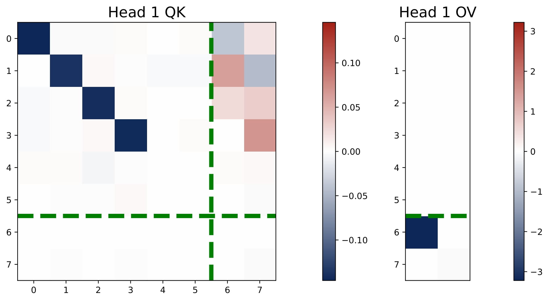
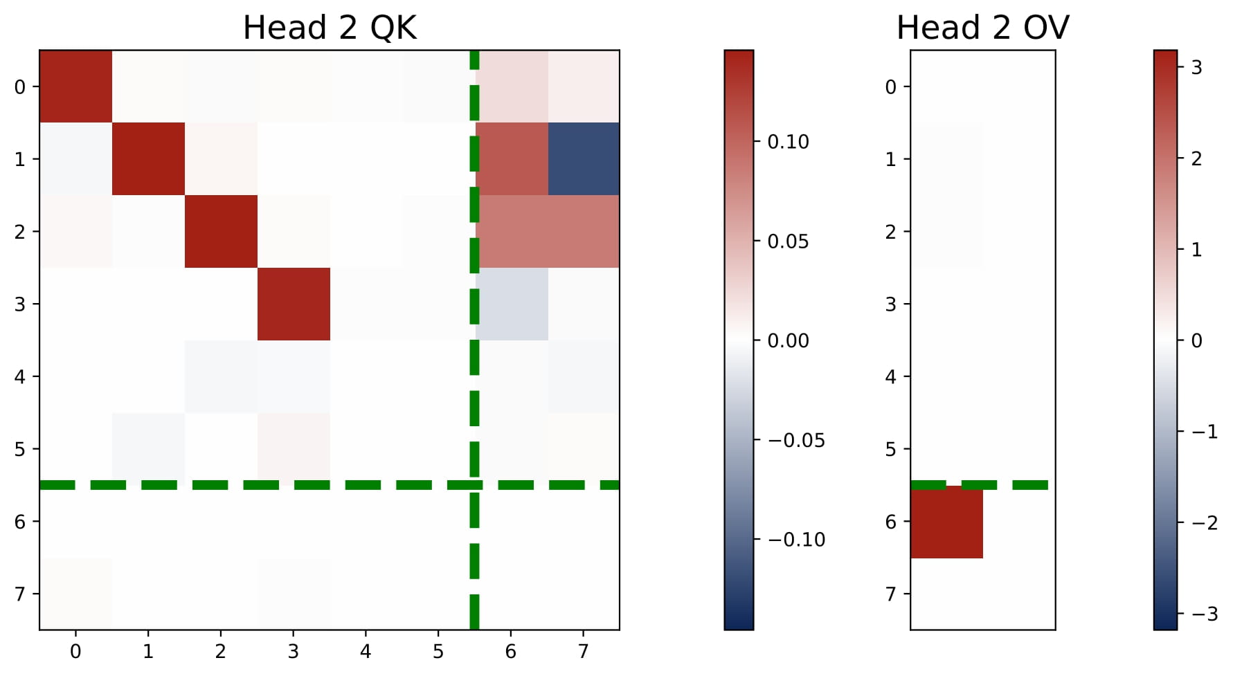
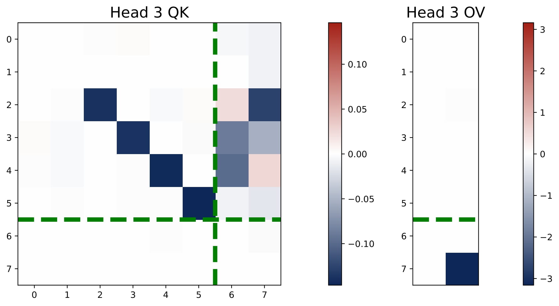
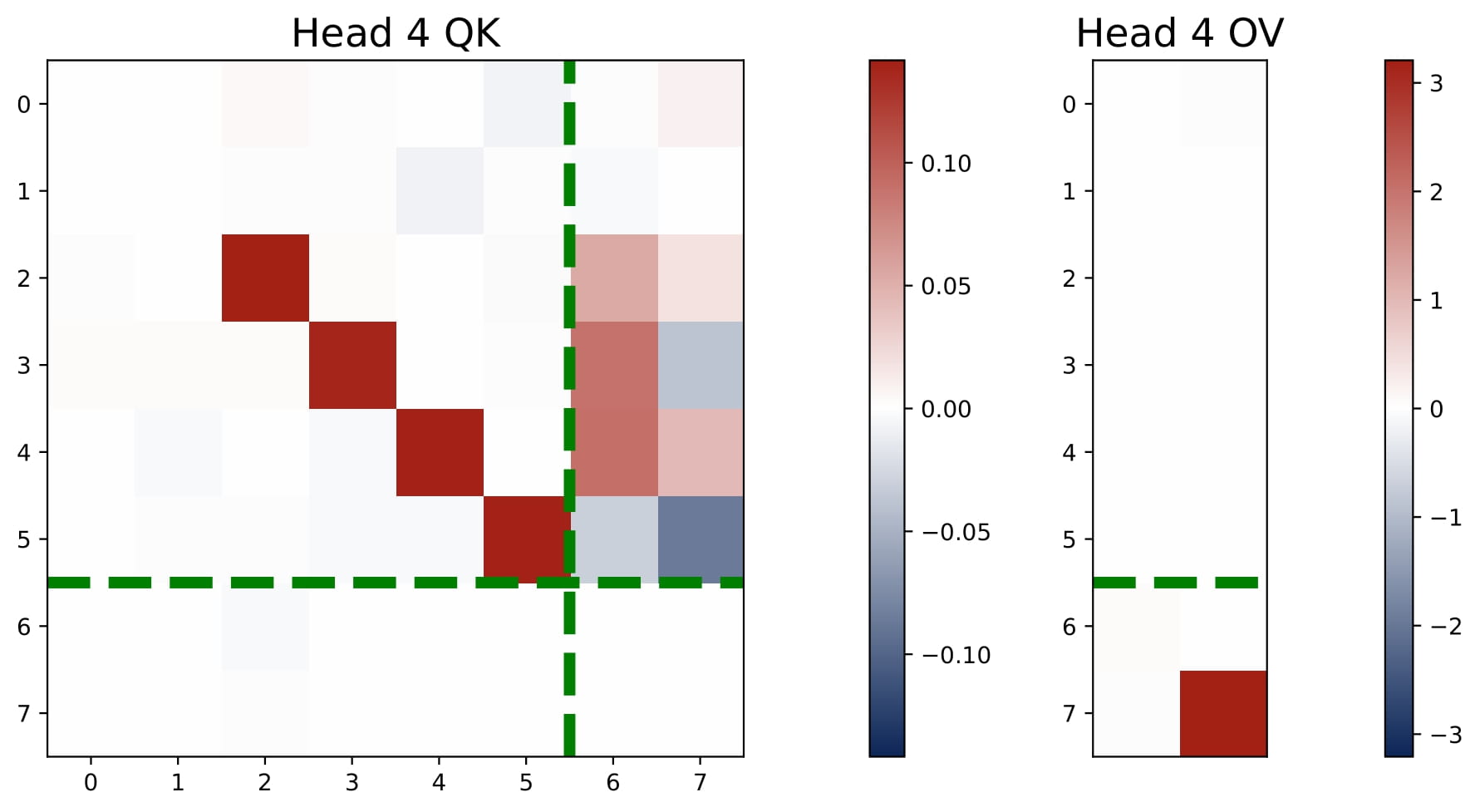
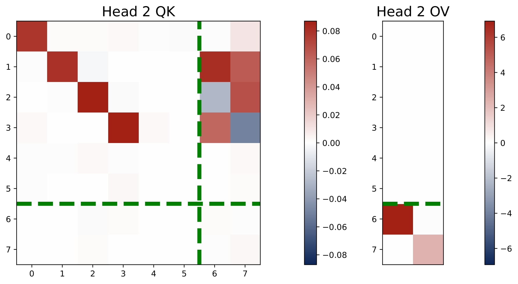
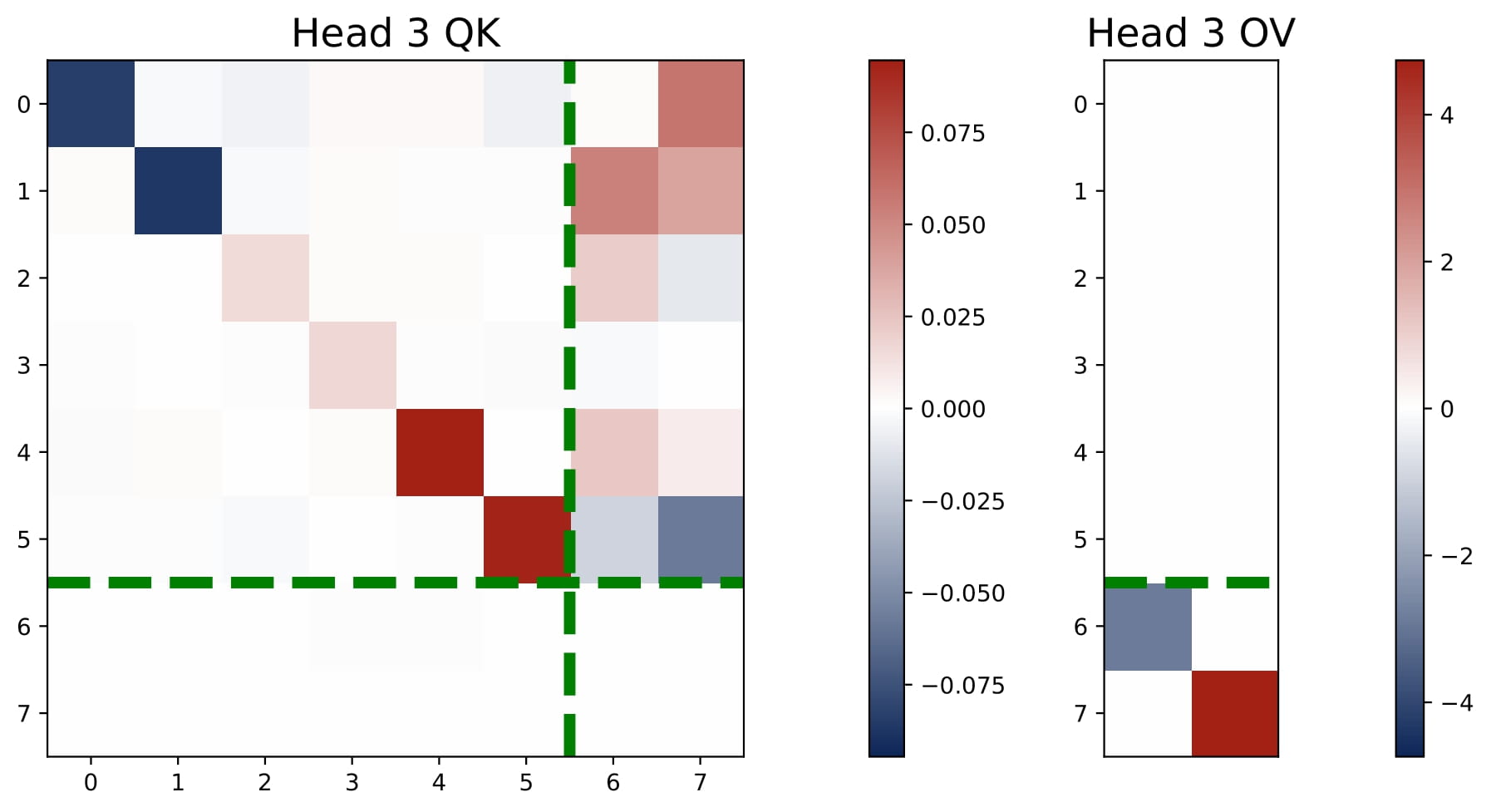
- $2 < H < 2N$: We observe an intriguing superposition phenomenon. In Figure 3.5, we plot the heatmaps of the KQ and OV matrices of a three-head attention model. Head 3 shows an interesting superposition pattern: it is a negative head for Task 1 and a positive head for Task 2. Intuitively, superposition requires requires some heads to solve move than one task simultaneously, which means that we may observe $\omega^{(h)}$ that have both positive and negative values.
Interestingly, three-head attention learns the same predictor as the four-head attention, i.e., it learns $N$ separate debiased GD predictors for the multi-task problem. But superposition enables the transformer model to implement these predictors in a more compact manner, using less heads. Here, each head is used to solve both tasks, but the aggregated effect is that the model can approximate the performance of the $N$ separate debiased GD predictors! As we detail in the paper, the learned KQ and OV circuits also reflect the structure of the support sets $\{ \mathcal{S}_n\}_{n\in[N]}$ and they satisfy certain conditions that enables the more compact implementation.
We only study a toy case with $H=3$ and $N=2$. We believe that the superposition phenomenon is a general phenomenon that occurs when $2 In this section, we focus on the the single-task and isotropic case and present the theoretical explanations for the learned multi-head attention model. Since the transformer’s KQ and OV circuits settle into a diagonal-only and last-entry-only structure early in training, we can reparameterize the model in terms of $(\omega,\mu)$. This simplified view captures the core learning behavior: the final prediction $\hat{y}_q$ can be computed based on the scaling parameters of the KQ and OV circuits, namely $\omega$ and $\mu$. Now we can regard the population risk of ICL as a function of $\omega$ and $\mu$.
We derive an approximation loss, which is more amenable for theoretical analysis. In fact, the approximation is accurate when the sample size $L$ is sufficiently large.
Empirical evidence shows that this approximation closely tracks the true loss landscape even as $\omega$ and $\mu$ change throughout training. Starting from small random initialization, the attention parameters converge in two main stages under gradient descent in terms of the approximate loss where Stage I establishes the sign-matching and zero-sum OV pattern such that driven by low-order gradient terms by applying the Taylor expansion to $\exp(d\omega\omega^\top)$ in the gradient dynamics. Specifically, we can write the gradient updates as: \begin{align*}
\mu_{t+1}\leftarrow&\mu_t+2\eta\cdot\underbrace{\left(1-\big(1+(1+\sigma^2)\cdot d{L}^{-1}\big)\cdot\langle\mu_t,\omega_t\rangle\right)\cdot{\omega_t}}_{\text{Sign-Matching Term}}\notag\\
&\qquad -2\eta\cdot(1+\sigma^2)\cdot L^{-1}\cdot\Big(\underbrace{{\langle\mu_t,\mathbf{1}_H\rangle}\cdot\mathbf{1}_H}_{\text{Zero-Sum OV Term}}+\underbrace{\sum_{k=2}^\infty \frac{d^k}{k!}\cdot\langle\mu_t,\omega_t^{\odot k}\rangle\cdot\omega_t^{\odot k}}_{\text{High-Order Terms}}\Big).
\end{align*} \begin{align*}
\omega_{t+1}\leftarrow&\omega_t+2\eta\cdot\underbrace{\left(1-\big(1+(1+\sigma^2)\cdot d{L}^{-1}\big)\cdot\langle\mu_t,\omega_t\rangle\right)\cdot{\mu_t}}_{\text{Sign-Matching Term}}\notag\\
&\qquad -2\eta\cdot(1+\sigma^2)\cdot L^{-1}\cdot\underbrace{\sum_{k=2}^\infty \frac{d^k}{(k-1)!}\cdot\langle\mu_t,\omega_t^{\odot k}\rangle\cdot\mu_t\odot\omega_t^{\odot k-1}}_{\text{High-Order Terms}}.
\end{align*}
Here $\omega^{\odot k}$ denote the $k$-th order Hadamard product of $\omega$, which produces a vector whose $j$-th entry is $\omega_j^k$ for all $j$. In the first stage, the gradient dynamics are driven by the low-order terms. Eventually, gradient descent will move to some $\omega$ and $\mu$ such that the low order terms are approximately zero. Zero-Sum OV Term: The term $\langle\mu_t,\mathbf{1}_H\rangle \cdot\mathbf{1}_H$ promotes the pattern of zero-sum OV. When this pattern emerges, this term is zero. Sign-Matching Terms: The two sign-matching terms leads to the emergence of the sign-matching pattern. Consider the update with these terms: \begin{align*}
\mu_{t+1}\leftarrow&\mu_t+2\eta\cdot\underbrace{\left(1-\big(1+(1+\sigma^2)\cdot d{L}^{-1}\big)\cdot\langle\mu_t,\omega_t\rangle\right)\cdot{\omega_t}}_{\text{Sign-Matching Term}}\\
\omega_{t+1}\leftarrow&\omega_t + 2\eta\cdot\underbrace{\left(1-\big(1+(1+\sigma^2)\cdot d{L}^{-1}\big)\cdot\langle\mu_t,\omega_t\rangle\right)\cdot{\mu_t}}_{\text{Sign-Matching Term}} .
\end{align*}
Here $\omega_t$ and $\mu_t$ update in each other’s directions, and thus eventually they will have the same sign. Once the previous two patterns emerge, in Stage II we need to further consider the high-order terms. The pattern of homogeneous KQ scaling emerges, which states that To see this, we apply Taylor expansion to the approximate loss function $\tilde{\mathcal{L}}$ and get Solution Manifold: With these patterns, the heads split into three groups—positive, negative, and dummy—and the resulting parameters $(\omega,\mu)$ lie on a solution manifold where
\begin{align}
\mathscr{S}_\gamma & =\Big\{(\omega,\mu)\subseteq\mathbb{R}^H :\omega^{(h)}= \gamma\cdot\mathrm{sign}(\mu^{(h)}),\quad
\sum_{h\in\mathcal{H}_{+}}\mu^{(h)}=-\sum_{h\in\mathcal{H}_{-}}\mu^{(h)}=\mu_\gamma\Big\},\\
&\text{where}\quad\mu_\gamma=\left(\gamma^2+(1+\sigma^2)\cdot L^{-1}\cdot\sinh(d\gamma^2)\right)^{-1}\cdot\gamma/2.
\end{align}
The specific scale $\gamma$ is sensitive to optimization details, e.g., learning rate. But theoretically, we can show that the optimal $\gamma$ is $0^{+}$, which gives rise to the debiased GD estimator. Our experiments show that no matter how many heads the model has, it consistently acquires diagonal-only KQ and last-entry-only OV circuits. For $H \ge 2$, the heads split into three groups—positive, negative, and dummy—and effectively approximate a gradient-descent-style solution. Specifically: Equivalent to Two-Head Form. Even in higher-head models, only the positive and negative heads contribute to the final predictor, which can be expressed exactly as a two-head model with parameters $\omega_{\mathrm{eff}} = (\gamma, -\gamma)$ and $\mu_{\mathrm{eff}} = (\mu_\gamma, -\mu_\gamma)$. For small $\gamma$, this predictor approximates a debiased GD predictor:
\begin{align*}
\hat{y}_q & = \mu_{\gamma}\cdot\biggl( \sum_{\ell=1}^L \frac{y_\ell\cdot\exp(\gamma\cdot x_\ell^\top x_q)}{\sum_{\ell=1}^L \exp(\gamma\cdot x_\ell^\top x_q)} -
\sum_{\ell=1}^L\frac{y_\ell\cdot\exp(-\gamma\cdot x_\ell^\top x_q)}{\sum_{\ell=1}^L\exp(-\gamma\cdot x_\ell^\top x_q)} \bigg)\\
&\approx\frac{{2\mu_\gamma\gamma}}{L}\cdot\sum_{\ell=1}^L y_\ell \cdot \bar{x}_\ell^\top x_q\quad\text{with}\quad\bar{x}_\ell=x_\ell-{L}^{-1}\cdot \sum_{\ell=1}^L x_\ell.
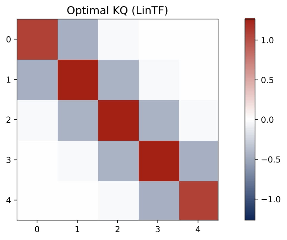
\end{align*} Debiased GD vs. Vanilla GD. When $L \gg d$, debiased GD coincides with vanilla GD since $\mathbb{E}[x_\ell]=0$, so multi-head softmax attention becomes equivalent to linear attention studied in prior work. Single-Head vs. Multi-Head. Single-head attention behaves like a kernel estimator (e.g., a Nadaraya–Watson regressor with a Gaussian RBF kernel and $\\|x_\ell\\|_2$ fixed). By contrast, multi-head attention implements a parametric form akin to GD, leading to better statistical performance for in-context linear regression. Approximation, Optimality, and Bayes Risk. The arguments above can be formally summarized in the following theorem. Theorem 1. Consider the parameter space $\overline{\mathscr{S}} \supseteq \mathscr{S}^*$ defined by Consider $\theta = (\omega,\mu)\in \overline{\mathscr{S}}$, and let $\sum\_{h\in \mathcal{H}\_{+}}\mu^{(h)} = \mu\_{+}$ and $\sum\_{h\in \mathcal{H}\_{-}}\mu^{(h)} = \mu\_{-}$. Then: where $\mathsf{BayesRisk} \_{\xi,\sigma^2}$ denotes the limiting Bayes risk. Recent work has explored linear transformers (e.g., Von Oswald et al., 2023
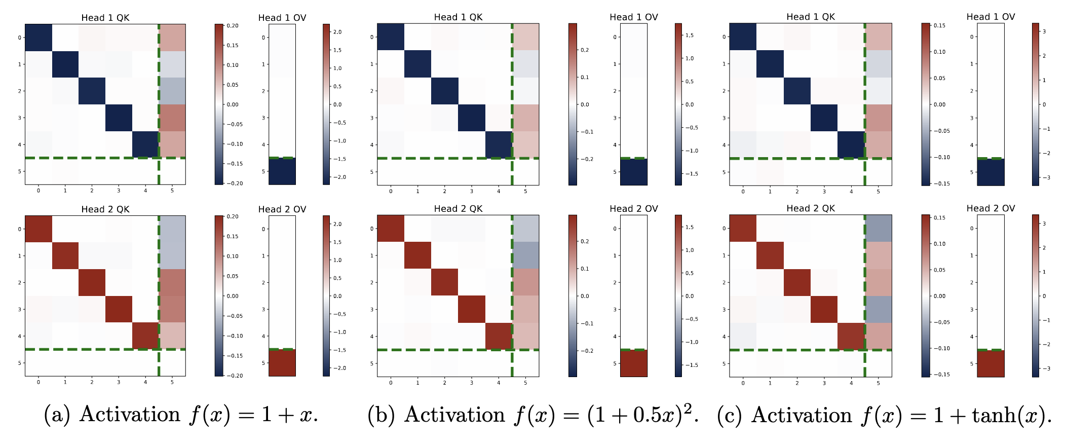
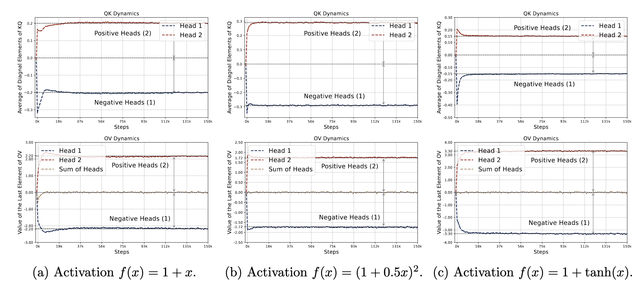
), which remove the nonlinearity and causal mask. Concretely, linear attention is defined as When applied to linear regression tasks, such a single-head linear transformer can learn the same one-step gradient descent solution as its softmax-based counterpart. However, softmax attention offers two key advantages: We found that the previous findings can also be extended to more general types of activations. We replaced the exponential function in softmax with alternative “normalized activations”:
$\sigma:\mathbb{R}^d\mapsto\mathbb{R}^d$ defined by letting $\sigma(\nu)\_i=f(\nu_i)/\sum\_{j=1}^df(\nu_j)$ for all $i\in[d]$,
where $f(\cdot)$ is any univariate function satisfying $f(x)\approx 1 + C_f\cdot x$ for small $x$. We tested three such families: (1) $f(x)=1+Cx$,
(2) $f(x)=(1+Cx)^2$, and (3) $f(x)=1+\tanh(x)$,
all of which share the first-order property $f(x)\approx 1 + C_f\cdot x$.
We have the following key observations: \begin{align*}
\hat{y}_q &= \| \mu\|_{\infty} \cdot \biggl( \sum_{\ell=1}^L \frac{y_\ell\cdot{f} ( \| \omega\|_{\infty} \cdot x_\ell^\top x_q)} {\sum_{\ell=1}^L{f}(\| \omega\|_{\infty} \cdot x_\ell^\top x_q)} - \sum_{\ell=1}^L \frac{y_\ell\cdot {f} (-| \omega|_{\infty}\cdot x_\ell^\top x_q)}{\sum_{\ell=1}^L {f}(-\| \omega\|_{\infty}\cdot x_\ell^\top x_q)} \bigg), \notag\\
&\approx \frac{\eta_{\mathsf{eff}} } {L} \sum_{\ell=1}^ L y_{\ell} \cdot \bar x_{\ell}^\top x_q, \qquad \textrm{where}
~~ \eta_{\mathsf{eff}} = 2 {C_{f}}\cdot \| \omega\|_{\infty} \cdot \| \mu\|_{\infty}
\end{align*} We studied how multi-head softmax attention models learn in-context linear regression, revealing emergent structural patterns that drive efficient learning.
Our analysis reveals that trained transformers develop structured key-query (KQ) and output-value (OV) circuits, with attention heads forming opposite positive and negative groups.
These patterns emerge early in training and are preserved throughout the training process, enabling the transformers to approximately implement a debiased gradient descent predictor.
Additionally, we show that softmax attention generalizes better than linear attention to longer sequences during testing and that learned attention structures extend to non-isotropic and multi-task settings.
As for future work, some interesting directions include ICL with nonlinear regression data or transformer models with at least two layers.
Another intriguing problem is systematically demystifying the superposition phenomenon for multi-task ICL in the general case.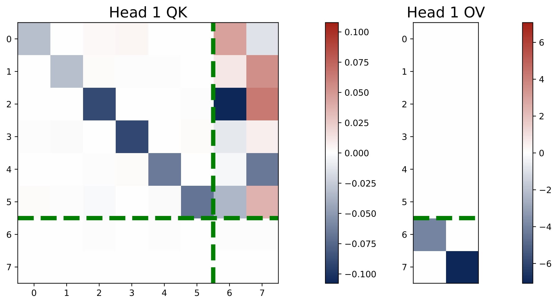
🔬 Mechanistic Interpretation
💎 Simplification and Approximate Loss
💎 Training Dynamics, Emerged Patterns, and Solution Manifold
\begin{align*}
\tilde{\mathcal{L}}(\omega_t,\mu_t)
&= \sigma^2+(1-\langle\mu_t,\omega_t\rangle)^2+(1+\sigma^2)\cdot L^{-1}\cdot\langle\mu_t,\mathbf{1}_H\rangle^2\\
&\qquad+(1+\sigma^2)\cdot L^{-1}\cdot\sum_{k=1}^\infty \frac{d^k}{k!}\cdot\langle\mu_t,\omega_t^{\odot k}\rangle^2.
\end{align*}
Using the nonnegativity of even terms and Holder’s inequality for odd terms, we have a lower bound for the Taylor series:
\begin{align}
\sum_{k=1}^\infty \frac{d^k}{k!}\cdot\langle\mu_t,\omega_t^{\odot k}\rangle^2&=\sum_{k\in{2q:q\in\mathbb{Z}^+}}\frac{d^k}{k!}\cdot\langle\mu_t,|\omega_t|^{\odot k}\rangle^2+\sum_{k\in{2q-1:q\in\mathbb{Z}^+}}\frac{d^k}{k!}\cdot\langle|\mu_t|,|\omega_t|^{\odot k}\rangle^2 \notag \\
&\geq\sum_{k\in{2q-1:q\in\mathbb{Z}^+}}\frac{d^k}{k!}\cdot|\mu_t|_1^{2(1-k)}\cdot\langle|\mu_t|,|\omega_t|\rangle^{2k},
\end{align}
The inequality becomes an equality when the following two conditions are satisfied.
First, the even terms are all equal to zero. Second, the inequality for the odd terms is actually an equality. Both these two conditions are satisfied when homogeneous KQ is true..
Therefore, the pattern of homogeneous KQ naturally emerges froms minimizing $\tilde{ \mathcal{L}}$.💎 Statistical Properties of Learned Multi-Head Attention
$$
\frac{\mathcal{E}(\hat{y}\_q^{\mathsf{gd}}(\eta^\ast))}{\mathsf{BayesRisk}\_{\xi,\sigma^2}}\leq 1+
\sigma^{-2} \cdot \big\\{(1+\xi\sigma^2)\cdot(1+\sigma^2+\xi^{-1})\big\\}^{-1},
$$📝 Discussion: Role of Softmax Activation
💎 Linear vs Softmax Attention
💎 Ablation Study: Activation Functions beyond Softmax
🎯 Conclusion
BibTex
@article{he2025context,
  title={In-Context Linear Regression Demystified: Training Dynamics and Mechanistic Interpretability of Multi-Head Softmax Attention},
  author={He, Jianliang and Pan, Xintian and Chen, Siyu and Yang, Zhuoran},
  journal={arXiv preprint arXiv:2503.12734},
  year={2025}
}