AUTHORS: Jianliang He, Leda Wang, Fengzhuo Zhang, Siyu Chen, Zhuoran Yang
AFFILIATIONS: Department of Statistics and Data Science, Yale University
LINKS: arXiv: 2606.02993 | GitHub: Code
Abstract
We prove that neural networks trained to compose elements of a finite group $G$ discover the irreducible representations of $G$ through gradient descent. Extending our prior work on modular addition (the cyclic group $\mathbb{Z}_p$), we show that the same spectral learning phenomenon generalizes to arbitrary finite groups, including non-Abelian ones. For general groups, we establish that each neuron’s Fourier coefficients converge to a single irreducible representation with rank-one rotational alignment, a matrix-valued generalization of the phase alignment observed in cyclic groups. For Abelian groups, we additionally prove diversification (uniform coverage of all irreducible representations) and characterize the exponential convergence rates via a lottery ticket mechanism. These results give a theoretical explanation for why neural networks learn harmonic analysis when trained on algebraic tasks.
1. Introduction and Motivation
In our prior work (He et al., 2026; see our blog post for a detailed exposition), we studied how neural networks learn modular addition: computing the sum of two integers modulo an odd number $p$. The task is simple: given $x$ and $y$ in $\{0, 1, \ldots, p-1\}$, predict $(x + y) \bmod p$. We trained a two-layer network and identified three core observations about the learned solution.
The three observations from modular addition (He et al., 2026):
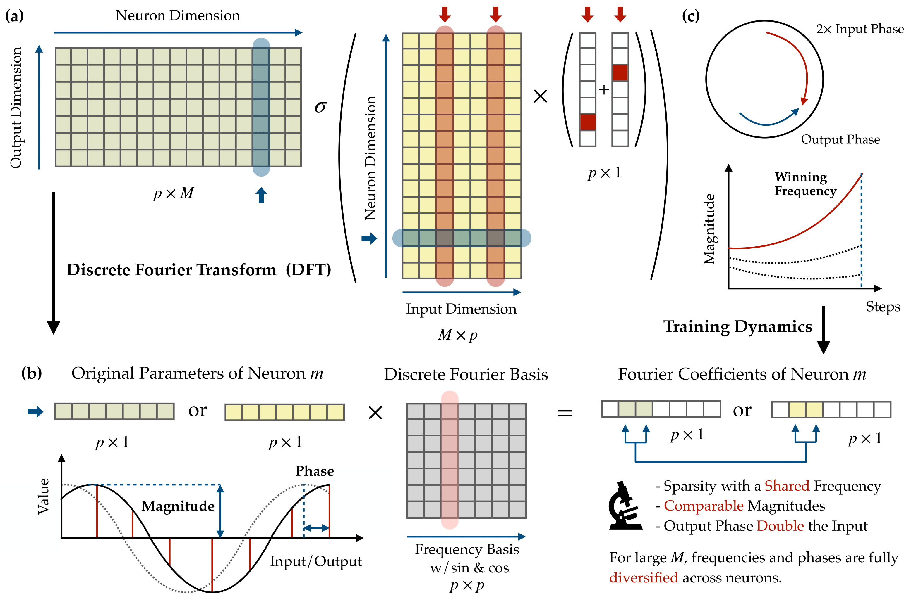
Single frequency. Each neuron’s weight vector is a cosine wave at a single Fourier frequency. If we apply the Discrete Fourier Transform to the learned input weight $\theta_m \in \mathbb{R}^p$, the result is extremely sparse: only one frequency $k_m$ has a nonzero coefficient, so $\theta_m[j] = \alpha_m \cos(2\pi k_m j / p + \phi_m)$.
Phase alignment. The input-layer phase $\phi_m$ and output-layer phase $\psi_m$ satisfy a precise doubled relationship: $\psi_m = 2\phi_m \pmod{2\pi}$. This coupling is not imposed by the architecture — it emerges from training.
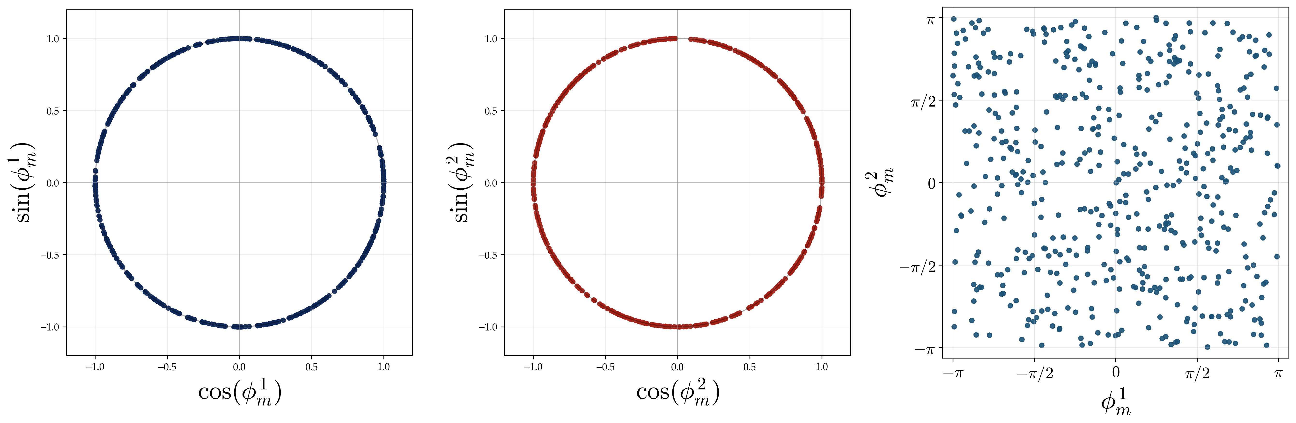
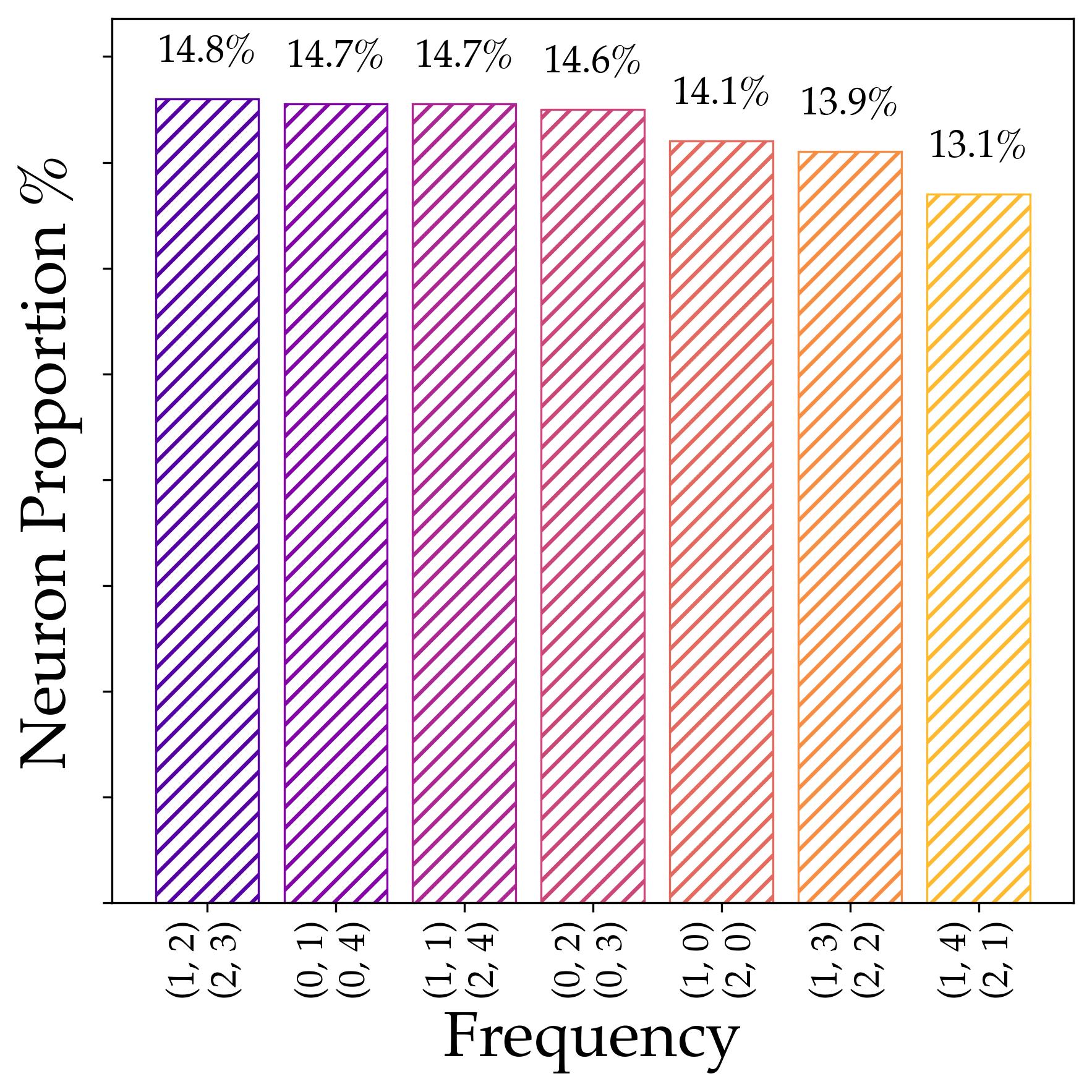
Diversification. The $M$ neurons collectively cover all $(p-1)/2$ non-trivial frequencies uniformly, and within each frequency group, the phases $\phi_m$ are spread evenly around the unit circle. This enables noise cancellation via a majority-voting mechanism that produces the correct answer.
These results raise two immediate questions:
Q1: What about general groups? Modular addition is the group operation of the cyclic group $\mathbb{Z}_p$. What changes when we move first to general Abelian groups, and then further to non-Abelian groups?
Q2: Why sine and cosine? Why does the network learn cosine waves specifically? Is this a coincidence tied to the cyclic structure, or is there a deeper reason?
The answer to Q2 is illuminating and motivates the entire paper. Cosines and sines are not an accident — they are the irreducible representations of the cyclic group $\mathbb{Z}_p$. For a cyclic group of order $p$, the irreducible representations are the characters $\chi_k(x) = e^{2\pi i k x / p}$, whose real and imaginary parts are $\cos(2\pi k x / p)$ and $\sin(2\pi k x / p)$. The network learns cosine waves because it is discovering the representation theory of the group it is computing on.
This realization suggests the general answer to Q1: for an arbitrary group $G$, the network should learn the irreducible representations of $G$ in their natural form. For Abelian groups, these are still one-dimensional (complex exponentials, producing cosines and sines). For non-Abelian groups, they become matrix-valued: a $d$-dimensional irreducible representation maps each group element to a $d \times d$ unitary matrix. The rest of this blog explains why gradient descent discovers these matrix representations.
Main Question: When a neural network learns to compose elements of an arbitrary finite group $G$ — including genuinely non-commutative groups — does it still discover the harmonic structure of $G$? If so, what form does this take?
There are two layers to this question. The first is the extension from cyclic groups $\mathbb{Z}_p$ to general Abelian groups $\mathbb{Z}_{n_1} \oplus \cdots \oplus \mathbb{Z}_{n_d}$. Here the Fourier transform is still scalar-valued because all irreducible representations are one-dimensional. The second layer is the leap to non-Abelian groups, where irreducible representations become matrix-valued and the scalar phase relationship $\psi = 2\phi$ no longer makes sense. What replaces it?
The answer is rank-one rotational alignment: a matrix-valued condition that reduces to phase alignment in the scalar (Abelian) case but captures a genuinely new phenomenon for non-Abelian groups. The network learns to compress each $d_\rho$-dimensional representation into a rank-one slice, a single “direction” within the representation space.
1.1 Summary of Contributions
Contribution 1: General Groups — Single Representation and Rank-One Alignment. For any finite group $G$, the network does not spread a neuron across many group features. During Stage I, each neuron selects one irreducible representation; if that representation is matrix-valued, the neuron uses only a rank-one slice of it; and the input/output Fourier blocks satisfy rotational alignment. In plain language: each neuron learns one spectral feature of the group, compresses it as much as possible, and aligns the two inputs with the output.
Contribution 2: Abelian Groups — Refined Population Law, Perfect Accuracy, and Rates. In the Abelian specialization, where every irreducible representation is a one-dimensional character, the paper proves a sharper statement than the general theorem: neurons diversify uniformly across non-trivial characters, their phases spread uniformly, and the resulting flawed indicator mechanism gives perfect prediction. This refined Abelian analysis also yields explicit exponential convergence rates and the lottery ticket dynamics.
2. From Cyclic Groups to General Abelian Groups
This section is the recap and technical bridge. The ordinary modular addition task is the cyclic case: $G=\mathbb{Z}_p$ and the label is $x\star y=(x+y)\bmod p$. The learned cosine waves in that setting are not an isolated trick; they are the real form of the one-dimensional irreducible representations of $\mathbb{Z}_p$. The paper reformulates this observation for arbitrary finite Abelian groups and then uses the same language as the bridge to non-Abelian groups.
For $\mathbb{Z}_p$, the characters are
$$ \rho_k(x)=\exp(2\pi\mathrm{i}kx/p),\qquad k=0,\dots,p-1. $$A real cosine feature is just the real part of a phase-shifted character:
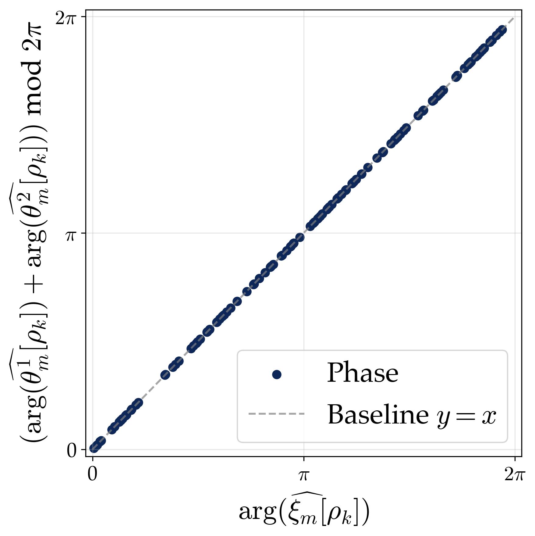
$$ \alpha\cos(2\pi kx/p+\phi)=\mathrm{Re}\big(\alpha e^{\mathrm{i}\phi}\rho_k(x)\big). $$Thus “single frequency” means that a neuron selects one character and its conjugate. The doubled-phase relation $\psi_m=2\phi_m$ is the shared-input Abelian case of the more general phase relation
$$ \arg(\hat{\xi}_m[\rho])= \arg(\hat{\theta}_m^1[\rho])+ \arg(\hat{\theta}_m^2[\rho]) \quad \bmod 2\pi. $$2.1 Generalizing the Setup
Modular addition is the group operation of the cyclic group $\mathbb{Z}_p$. We now extend the task to a general finite Abelian group, represented as a product of cyclic groups:
$$G_{\mathcal N} = \mathbb{Z}_{n_1} \oplus \mathbb{Z}_{n_2} \oplus \cdots \oplus \mathbb{Z}_{n_d}.$$This form is representative, not a restriction: by the Fundamental Theorem of Finite Abelian Groups, every finite Abelian group decomposes as a direct product of cyclic groups in this form. The group operation is component-wise addition:
$$(a_1, \ldots, a_d) \star (a_1', \ldots, a_d') = \bigl((a_1 + a_1') \bmod n_1,\; \ldots,\; (a_d + a_d') \bmod n_d\bigr).$$Concrete example: $\mathbb{Z}_3 \oplus \mathbb{Z}_5$. This group has order $3 \times 5 = 15$. Its elements are pairs $(a, b)$ with $a \in \{0, 1, 2\}$ and $b \in \{0, 1, 2, 3, 4\}$. The composition rule is $(a_1, b_1) \star (a_2, b_2) = ((a_1 + a_2) \bmod 3, (b_1 + b_2) \bmod 5)$. The network must learn a $15 \times 15$ “multiplication table” with $15^2 = 225$ input pairs.
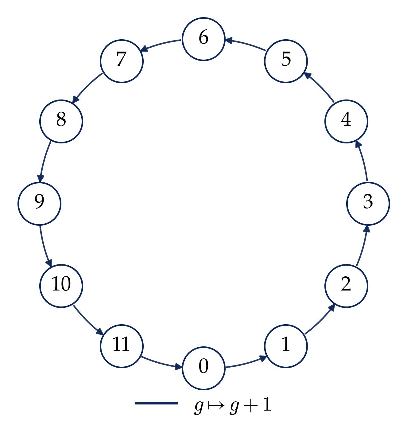
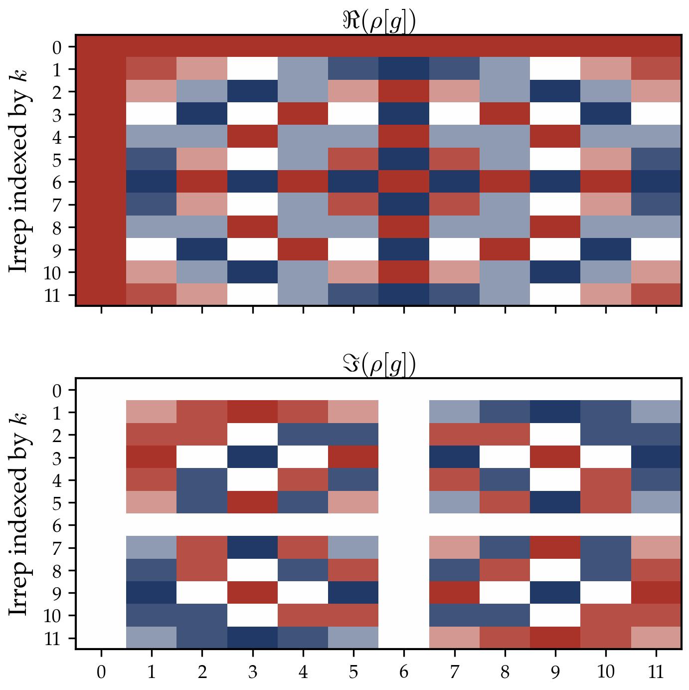
To visualize what a cyclic group and its Fourier basis look like, consider $\mathbb{Z}_{12}$:
2.2 Irreducible Representations of Abelian Groups
For Abelian groups, all irreducible representations are one-dimensional — they are characters, i.e., group homomorphisms $\rho: G \to \mathbb{C}^*$ satisfying $\rho(g_1 \star g_2) = \rho(g_1)\rho(g_2)$. For $G_{\mathcal N} = \mathbb{Z}_{n_1} \oplus \cdots \oplus \mathbb{Z}_{n_d}$, the characters are indexed by frequency tuples $k = (k_1, \ldots, k_d)$ with $k_j \in \{0, 1, \ldots, n_j - 1\}$:
$$\rho_k(a_1, \ldots, a_d) = \exp\!\left(2\pi \mathrm{i} \sum_{j=1}^d \frac{k_j a_j}{n_j}\right) = \prod_{j=1}^d \exp\!\left(\frac{2\pi \mathrm{i} k_j a_j}{n_j}\right).$$These are complex exponentials — the direct generalization of the Fourier basis $e^{2\pi \mathrm{i} k j / p}$ from the cyclic case. Expanding into real and imaginary parts gives cosines and sines. There are $|G| = n_1 \cdots n_d$ characters in total, of which one is trivial ($k = 0$).
Why complex exponentials? In our earlier $\mathbb{Z}_p$ work, we wrote everything in terms of cosines: $\theta_m[j] = \alpha \cos(\omega_k j + \phi)$. This is natural when $p$ is odd, because each non-trivial frequency $k$ is paired with its distinct conjugate $p - k$, and the real-valued weight vector combines the two: $\text{Re}(\hat{\theta} e^{i\omega_k j}) = \alpha \cos(\omega_k j + \phi)$. The complex exponential notation $e^{i\omega_k j}$ packages both the cosine and sine components into a single object. For general Abelian groups, the complex notation is cleaner because we work with multi-dimensional frequency tuples.
2.3 The Neural Network Model
We train on the complete composition table: every pair $(g_1,g_2)\in G_{\mathcal N}\times G_{\mathcal N}$ is observed, with label $g_1\star g_2$. Let $e_g\in\mathbb R^{|G|}$ denote the one-hot vector for group element $g$. The paper uses the two-layer logit model
$$ f_{\sf NN}(g_1,g_2;\Theta) =\frac{1}{M}\sum_{m=1}^M a_m\cdot \xi_m\cdot \sigma\!\left( \langle \theta_m^1,e_{g_1}\rangle+ \langle \theta_m^2,e_{g_2}\rangle \right) \in\mathbb R^{|G|}. $$Here $\Theta=\{(a_m,\xi_m,\theta_m^1,\theta_m^2)\}_{m\in[M]}$. The vectors $\theta_m^1,\theta_m^2\in\mathbb R^{|G|}$ are the two positional input embeddings, $\xi_m\in\mathbb R^{|G|}$ is the output embedding, $a_m>0$ is the neuron scaling factor, and $\sigma(x)=x^2$ throughout the paper. Since the inputs are one-hot, each vector $\nu\in\{\theta_m^1,\theta_m^2,\xi_m\}$ can also be viewed as a function $\nu:G\to\mathbb R$ via $\nu(g)=\langle \nu,e_g\rangle$. The vector $f_{\sf NN}(g_1,g_2;\Theta)$ is the logit over all output labels $j\in G$; prediction probabilities are obtained by applying softmax.
For the general group theorem, the two input embeddings are kept separate because the left and right operands need not play symmetric roles. In the refined Abelian analysis, the paper also studies the shared-input convention $\theta_m^1=\theta_m^2=:\theta_m$, which is natural when the group operation is commutative.
Two-stage training. The paper separates feature learning from scale optimization:
Stage I: directional training. Initialize
$$ a_m=a>0,\qquad (\theta_m^1(0),\theta_m^2(0),\xi_m(0)) \stackrel{\mathrm{iid}}{\sim} \mathrm{Unif}(\mathbb S^{|G|-1})^{\otimes 3}, \qquad m\in[M], $$with $a$ fixed and sufficiently small. Only the directional parameters evolve, constrained to the unit sphere:
$$ \partial_t\theta_m^\tau =-\bigl(I-\theta_m^\tau(\theta_m^\tau)^\top\bigr) \nabla_{\theta_m^\tau}\mathcal R(\Theta), \qquad \partial_t\xi_m =-\bigl(I-\xi_m\xi_m^\top\bigr) \nabla_{\xi_m}\mathcal R(\Theta), \qquad \tau\in\{1,2\}. $$The projection terms keep $\theta_m^1,\theta_m^2,\xi_m$ on $\mathbb S^{|G|-1}$. This is the stage in which the Fourier coefficients collapse to representations and align.
Stage II: scale optimization. Freeze $(\theta_m^1,\theta_m^2,\xi_m)$ at their Stage I values and optimize only the scales:
$$ \partial_t a_m=-\nabla_{a_m}\mathcal R(\Theta). $$This stage sharpens the softmax by increasing the margin of the correct class while keeping the learned spectral directions fixed.
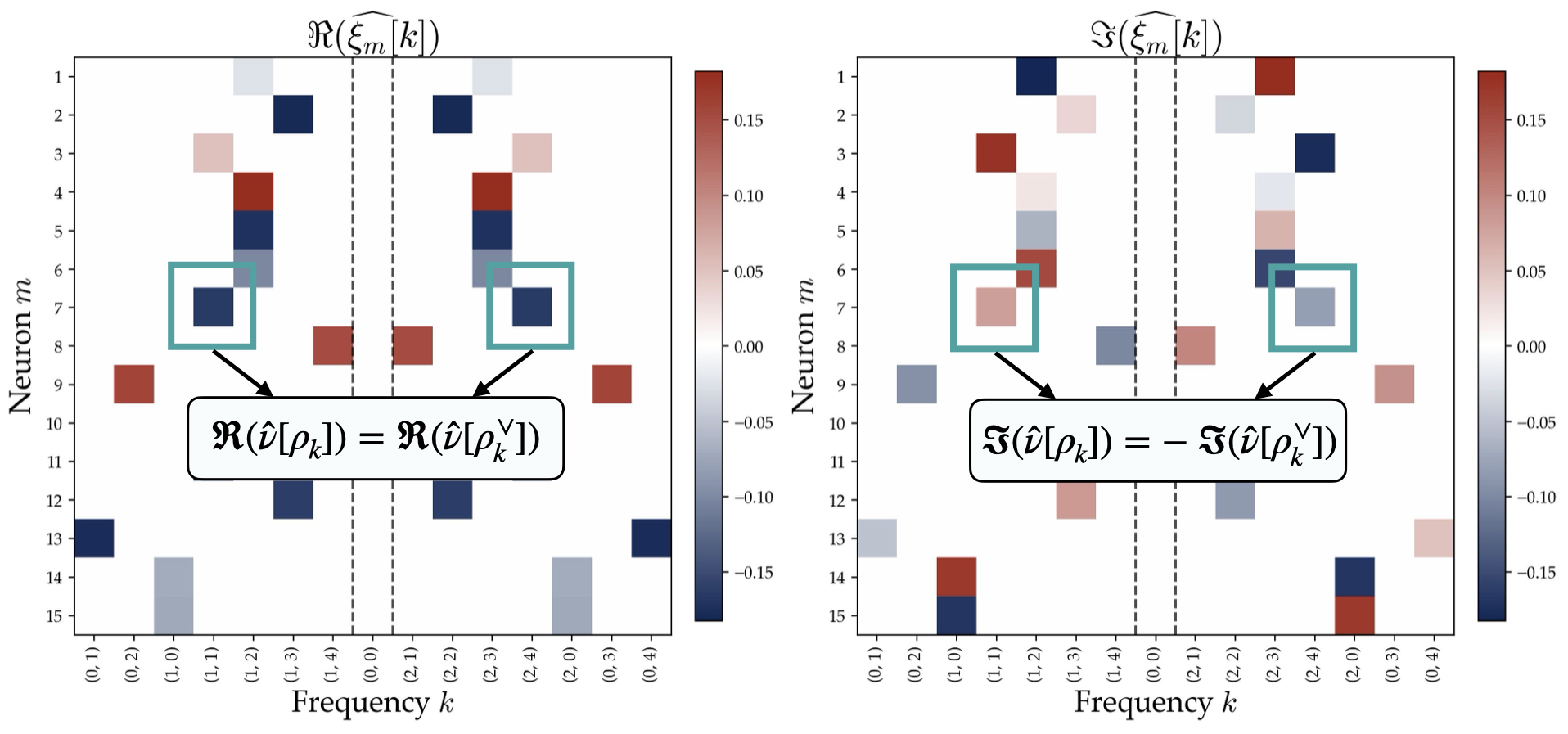
We verify the resulting spectral properties experimentally on $\mathbb{Z}_3 \oplus \mathbb{Z}_5$ (order 15, with $15 - 1 = 14$ non-trivial characters grouped into 7 conjugate pairs):
2.4 The Flawed Indicator Mechanism
How do these three properties combine to produce correct predictions? Through the same majority-voting mechanism as in $\mathbb{Z}_p$, now generalized.
What a single neuron computes. Consider a neuron $m$ that has selected representation $\check\rho_m$ with phase-aligned coefficients. Using $\sigma(x) = x^2$ and expanding $(\theta_m^1(g_1) + \theta_m^2(g_2))^2$, the neuron’s contribution to the logit at output position $j$ contains a signal term of the form $\mathrm{Re}(\check\rho_m(j(g_1\star g_2)^{-1}))$ plus phase-dependent terms.
The signal term peaks when $j = g_1 \star g_2$ because $\check\rho_m(\mathrm{id})=1$. The phase-dependent terms cancel at the population level because the learned phases are uniformly spread around the unit circle.
Summing over all neurons. After noise cancellation via diversification and summing over all non-trivial characters using the finite-group orthogonality relations, we obtain:
Proposition (Flawed Indicator Mechanism). In the Abelian population limit described in the paper, the mean-field predictor takes the form:
$$\mathcal F_{\sf NN}^{\mu}(g_1,g_2)_j \;\propto\; 2 \cdot \mathbf{1}\{j = g_1 \star g_2\} + \mathbf{1}\{j = g_1^2\} + \mathbf{1}\{j = g_2^2\} + \mathsf{const}.$$The correct answer $j = g_1 \star g_2$ gets coefficient 2, while the “ghost” peaks at $j = g_1^2$ and $j = g_2^2$ get coefficient 1. Since $2 > 1$, the correct answer always has the largest logit, and the softmax concentrates probability on the correct prediction.
The Abelian result is not only a statement about the final representation pattern. It also gives a dynamical story: phases align quickly, then a lottery-ticket competition selects the winning character inside each neuron. The paper quantifies both processes with exponential convergence rates.
3. The General Group Case: Non-Abelian Groups
We now turn to the main new contribution of this paper: extending the theory to arbitrary finite groups, including non-commutative ones. This is where qualitatively new mathematics enters.
3.1 Why Non-Abelian Groups Are Fundamentally Different
For non-Abelian groups, the representation theory undergoes a qualitative shift:
Matrix-valued representations. Irreducible representations are no longer one-dimensional characters. They are maps $\rho: G \to \text{GL}(\mathbb{C}^{d_\rho})$ where the dimension $d_\rho$ can be $2, 3, \ldots$ or more. The representation $\rho(g)$ is a $d_\rho \times d_\rho$ unitary matrix for each group element $g$.
Fourier coefficients are matrices. Instead of scalar Fourier coefficients $\hat{\theta}[\mathbf{k}] \in \mathbb{C}$, we now have matrix-valued coefficients $\hat{\theta}[\rho] \in \mathbb{C}^{d_\rho \times d_\rho}$.
Non-commutativity matters. For $G$ non-Abelian, $g_1 \star g_2 \neq g_2 \star g_1$ in general, so the left and right inputs play fundamentally different roles. The network must use two separate input embeddings.
Scalar phase alignment has no direct matrix analogue. The scalar condition $\arg(\hat{\xi}) = 2\arg(\hat{\theta})$ does not generalize to matrices: a $3 \times 3$ matrix does not have a single “phase.” What replaces it?
To make this concrete, consider the alternating group $A_4$ (the group of even permutations of 4 elements, order 12):
Key Questions: Does the single-representation phenomenon from modular addition still hold for arbitrary finite groups? If so, what structural condition on matrix-valued Fourier coefficients replaces scalar phase alignment?
3.2 Setup: Group Composition for General Groups
For a general finite group $(G,\star)$ of order $|G|$, the task is again full-table composition: predict $g_1\star g_2$ for every pair $(g_1,g_2)\in G\times G$. We use the same two-layer logit model and two-stage training procedure from the Abelian setup, but now the two input embeddings $\theta_m^1$ and $\theta_m^2$ are kept distinct. This asymmetry is essential: for non-commutative groups, left and right multiplication are different operations, so the network must represent the two operands separately.
3.3 The Fourier Transform on General Finite Groups
The Fourier transform on a general finite group replaces scalar frequencies with matrix-valued irreducible representations. A representation of $(G,\star)$ is a homomorphism
$$ \rho:(G,\star)\to(\mathrm{GL}(V_\rho),\cdot), \qquad \rho(g_1\star g_2)=\rho(g_1)\rho(g_2), $$where $V_\rho$ is a finite-dimensional complex vector space. The representation is irreducible if $V_\rho$ has no non-trivial invariant subspace under all matrices $\rho(g)$.
Let $\mathrm{Irr}(G)$ denote a complete set of irreducible unitary representations of $G$. For each $\rho\in\mathrm{Irr}(G)$, the paper fixes an orthonormal basis of $V_\rho$, so we identify $\rho(g)$ with a unitary matrix in $\mathbb C^{d_\rho\times d_\rho}$, where $d_\rho=\dim V_\rho$. These dimensions satisfy
$$ \sum_{\rho\in\mathrm{Irr}(G)}d_\rho^2=|G|. $$For Abelian groups all $d_\rho=1$, so the irreducible representations are scalar characters. For non-Abelian groups some $d_\rho>1$, and the Fourier coefficients become matrix blocks.
For any function $\nu: G \to \mathbb{R}$, its Fourier transform at representation $\rho$ is the $d_\rho \times d_\rho$ matrix:
$$\hat{\nu}[\rho]=\frac{1}{|G|}\sum_{g\in G}\nu(g)\rho(g^{-1})\in\mathbb C^{d_\rho\times d_\rho}.$$Fourier inversion reconstructs $\nu$:
$$\nu(g)=\sum_{\rho\in\mathrm{Irr}(G)}d_\rho\cdot\mathrm{tr}\big(\hat{\nu}[\rho]\rho(g)\big).$$This is the paper’s normalization. In this basis, the general group DFT decomposes a real vector $\nu\in\mathbb R^{|G|}$ into one block $\hat\nu[\rho]\in\mathbb C^{d_\rho\times d_\rho}$ for each irreducible representation. The dimension identity above says that the block sizes exactly account for the original $|G|$ degrees of freedom.
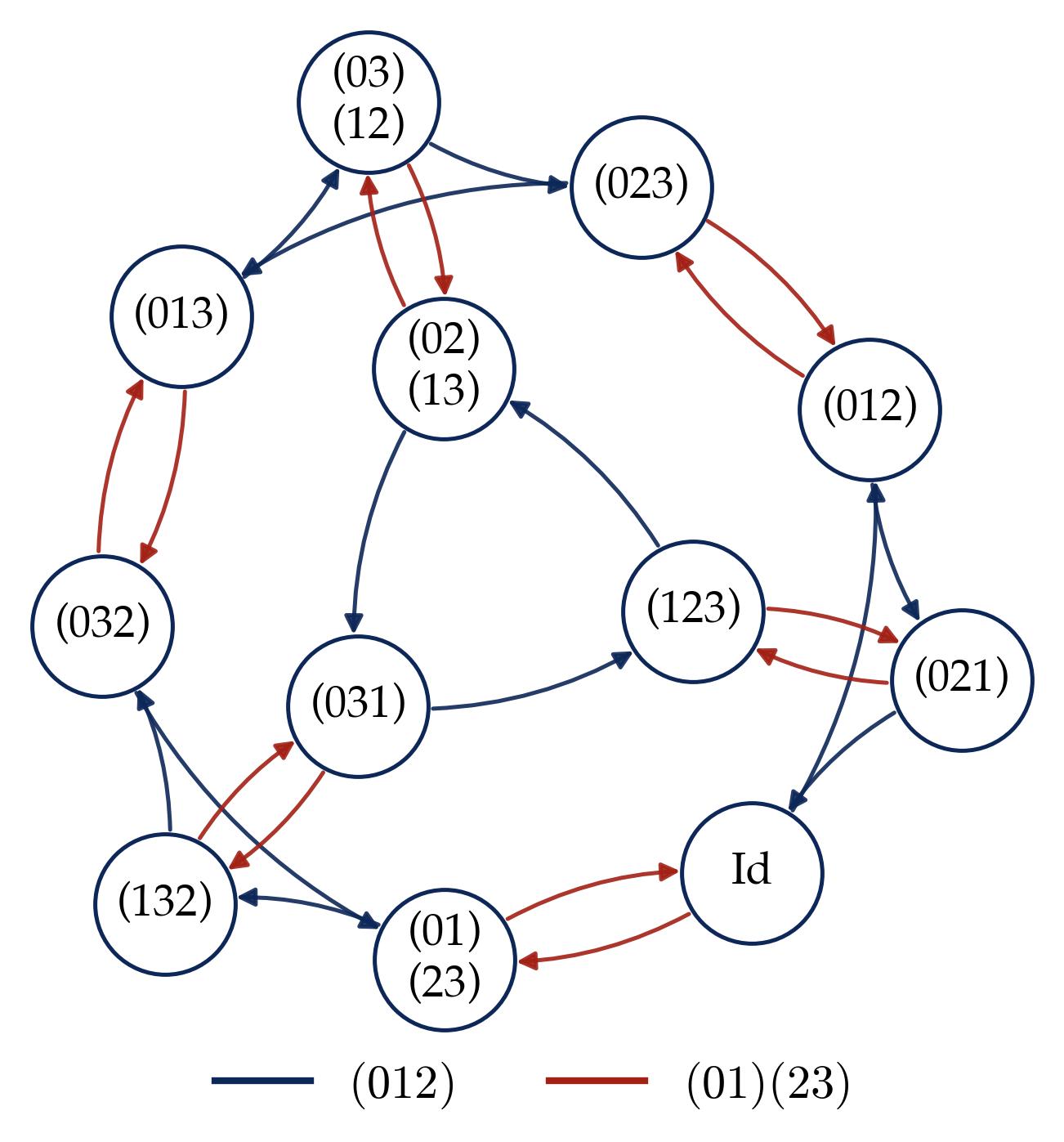
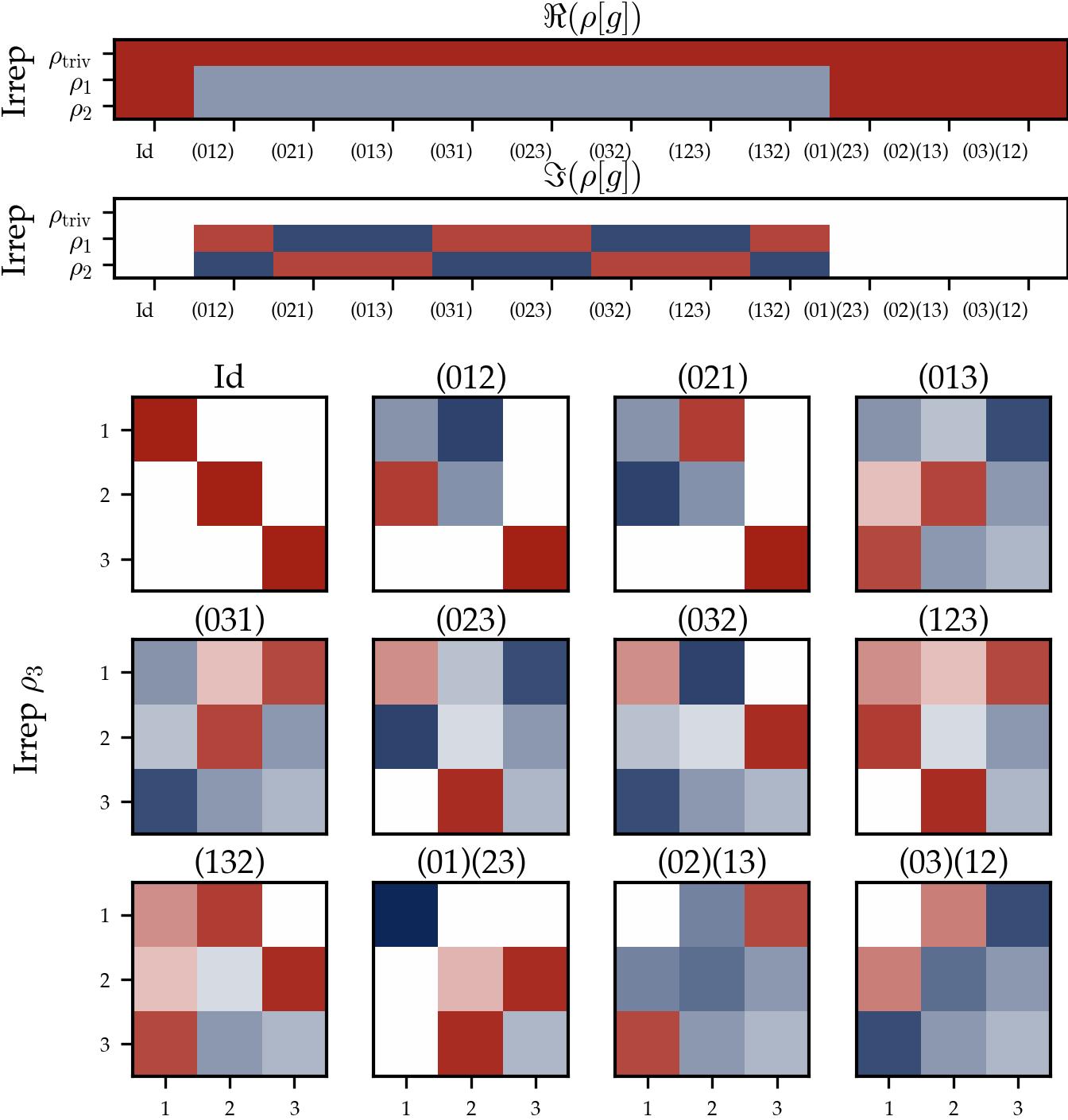
Concrete example: $C_7 \rtimes C_3$ (the Frobenius group of order 21). This is a semidirect product of the cyclic group of order 7 and the cyclic group of order 3. It is generated by two elements $x$ (order 7) and $y$ (order 3) subject to the relation $y x y^{-1} = x^2$ — that is, conjugation by $y$ acts on the normal subgroup $C_7$ by squaring. The group elements can be written as $x^a y^b$ with $a \in \{0, \ldots, 6\}$ and $b \in \{0, 1, 2\}$, and the multiplication rule is:
$$(x^a y^b) \star (x^{a'} y^{b'}) = x^{a + 2^b a' \bmod 7}\, y^{(b + b') \bmod 3}.$$Note the non-commutativity: the exponent $2^b a'$ twists the left factor depending on $b$. The group is a useful test case because it has a compact semidirect-product description while still requiring genuine 3D matrix-valued irreducible representations. It has five irreducible representations:
- Three 1-dimensional: the trivial $\rho_1$, and two others $\rho_2, \rho_3$ that are characters of the quotient $G/C_7 \cong C_3$ (they “see” only the $y$-component).
- Two 3-dimensional: $\rho_4$ and $\rho_5$, which are genuine matrix representations that mix the $x$ and $y$ components.
The dimension formula $\sum_i d_i^2 = |G|$ checks out: $1^2 + 1^2 + 1^2 + 3^2 + 3^2 = 1 + 1 + 1 + 9 + 9 = 21$.
For each neuron $m$, the Fourier transform gives: three $1 \times 1$ blocks (scalars) and two $3 \times 3$ blocks (matrices) — a total of $3 \cdot 1 + 2 \cdot 9 = 21$ parameters, matching the ambient dimension $|G| = 21$.
3.4 Main Result: Single Representation with Rank-One Rotational Alignment
We can now state the main theorem. The key message is simple: each neuron picks one representation and uses it in the most compressed way possible.
Theorem (Global Convergence of Spectral Patterns). Consider the Stage I projected gradient flow under the approximate small-logit risk. For every neuron $m$, there exists a non-trivial irreducible representation $\check\rho_m\in\mathrm{Irr}(G)_{\neq1}$ such that, almost surely as $t\to\infty$, the following hold:
(i) Single Representation. For all $\rho\in\mathrm{Irr}(G)\setminus\mathrm{orb}(\check\rho_m)$ and every $\nu\in\{\xi_m,\theta_m^1,\theta_m^2\}$, the Fourier block vanishes: $\hat\nu[\rho]\to0_{d_\rho\times d_\rho}$. Here $\mathrm{orb}(\rho)=\{\rho,\rho^\vee\}$. Consequently, each parameter is reconstructed from the active orbit:
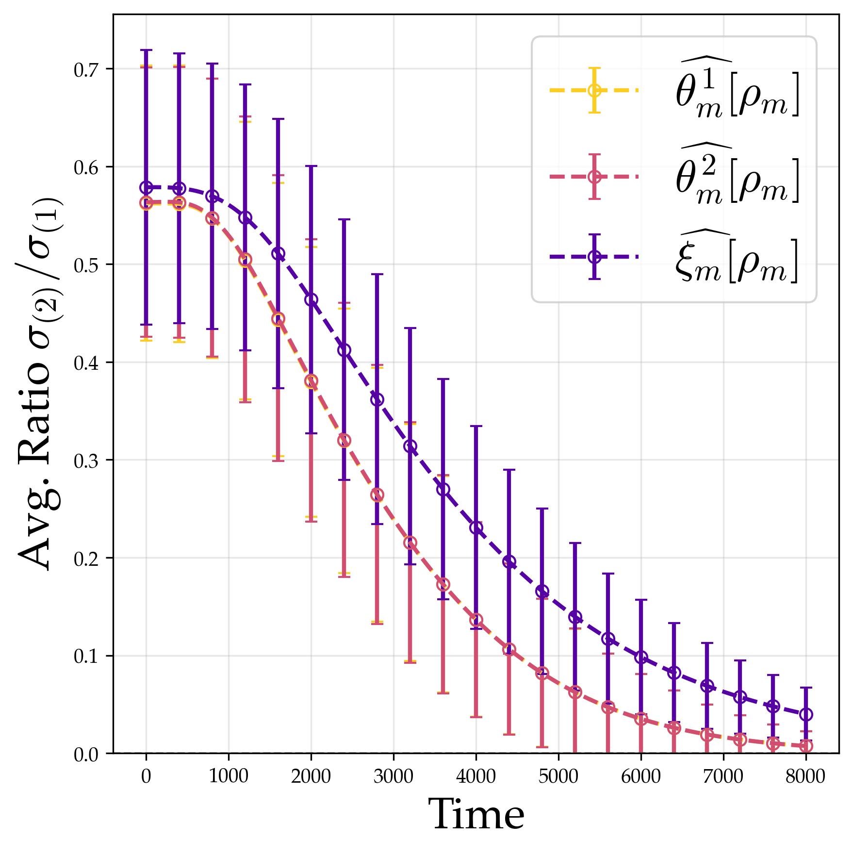
$$ \nu(g)=d_{\check\rho_m}\cdot|\mathrm{orb}(\check\rho_m)|\cdot \mathrm{Re}\big(\mathrm{tr}(\hat\nu[\check\rho_m]\check\rho_m(g))\big), \qquad \nu\in\{\theta_m^1,\theta_m^2,\xi_m\}. $$(ii) Rank-One Rotational Alignment. The surviving Fourier coefficient matrices are all rank one, and the output block is proportional to the product of the two input blocks:
$$ \mathrm{rank}(\hat{\theta}_m^1[\rho]) =\mathrm{rank}(\hat{\theta}_m^2[\rho]) =\mathrm{rank}(\hat{\xi}_m[\rho])=1, $$and, for active $\rho\in\mathrm{orb}(\check\rho_m)$,
$$ \hat{\xi}_m[\rho]\propto_+\hat{\theta}_m^2[\rho]\hat{\theta}_m^1[\rho],\qquad \hat{\theta}_m^1[\rho]\propto_+(\hat{\theta}_m^2[\rho])^*\hat{\xi}_m[\rho],\qquad \hat{\theta}_m^2[\rho]\propto_+\hat{\xi}_m[\rho](\hat{\theta}_m^1[\rho])^*. $$Here $A\propto_+B$ means $A=cB$ for some positive real scalar $c$.
Interpretation.
Think of the group Fourier transform as decomposing each neuron’s weight vector into “channels,” one per irreducible representation. For the Frobenius group $C_7 \rtimes C_3$, there are five channels: three scalar channels (for the 1D representations) and two matrix channels (for the 3D representations). The theorem says:
Only one channel is active. After training, each neuron concentrates all its energy in a single channel; all others are silent. A neuron either selects one of the 1D representations (so its weight is a scalar function) or one of the 3D representations (so its weight encodes a $3 \times 3$ matrix). This is the exact analogue of “single frequency” from the cyclic case.
The active channel is maximally compressed. Even within a 3D representation (which offers a $3 \times 3 = 9$-dimensional space of possible matrices), the neuron uses only a rank-one matrix: an outer product $\mathbf{u}\mathbf{v}^\dagger$ specified by just two vectors. It picks a single “direction” through the representation space rather than using the full 9 degrees of freedom.
The three layers are coherently aligned. The output matrix $\hat{\xi}_m[\rho]$ is positively proportional to the product $\hat{\theta}_m^2[\rho]\hat{\theta}_m^1[\rho]$, and the two cyclic companion relations also hold. This is the matrix version of phase alignment. When $d_\rho = 1$ (scalars), the first relation reduces to $\arg(\hat{\xi}_m[\rho]) = \arg(\hat{\theta}_m^1[\rho]) + \arg(\hat{\theta}_m^2[\rho])$.
Proof sketch. The proof starts by moving Stage I into the Fourier domain. In the small-logit regime, the projected gradient flow for each neuron decouples from the other neurons and becomes Riemannian gradient ascent on the trilinear spectral energy
$$ \Omega_m=\sum_{\rho\in\mathrm{Irr}(G)_{\neq1}}d_\rho\cdot\mathrm{tr}\big((\hat{\xi}_m[\rho])^*\hat{\theta}_m^2[\rho]\hat{\theta}_m^1[\rho]\big), $$subject to the norm constraints inherited from $\theta_m^1,\theta_m^2,\xi_m\in\mathbb S^{|G|-1}$. The product order $\hat{\theta}_m^2[\rho]\hat{\theta}_m^1[\rho]$ records the order of group composition inside the Fourier transform.
Because this energy is trilinear, holding two Fourier blocks fixed pushes the third block to align with their matrix product. Thus any positive-energy stable equilibrium must satisfy
$$ \hat{\xi}_m[\rho]\propto_+\hat{\theta}_m^2[\rho]\hat{\theta}_m^1[\rho],\qquad \hat{\theta}_m^1[\rho]\propto_+(\hat{\theta}_m^2[\rho])^*\hat{\xi}_m[\rho],\qquad \hat{\theta}_m^2[\rho]\propto_+\hat{\xi}_m[\rho](\hat{\theta}_m^1[\rho])^*. $$The main technical challenge is excluding non-target equilibria. The paper classifies critical points by energy sign, representation support, and rank. Negative-energy and trivial zero-energy cases occur only on exceptional initialization sets; non-degenerate zero-energy cases and higher-rank positive-energy cases are strict saddles. A Riemannian center-stable-manifold argument then shows that random initialization almost surely avoids those unstable sets. What remains are precisely the stable positive-energy equilibria: one active irrep orbit, rank-one Fourier blocks, and the cyclic proportionality relations above.
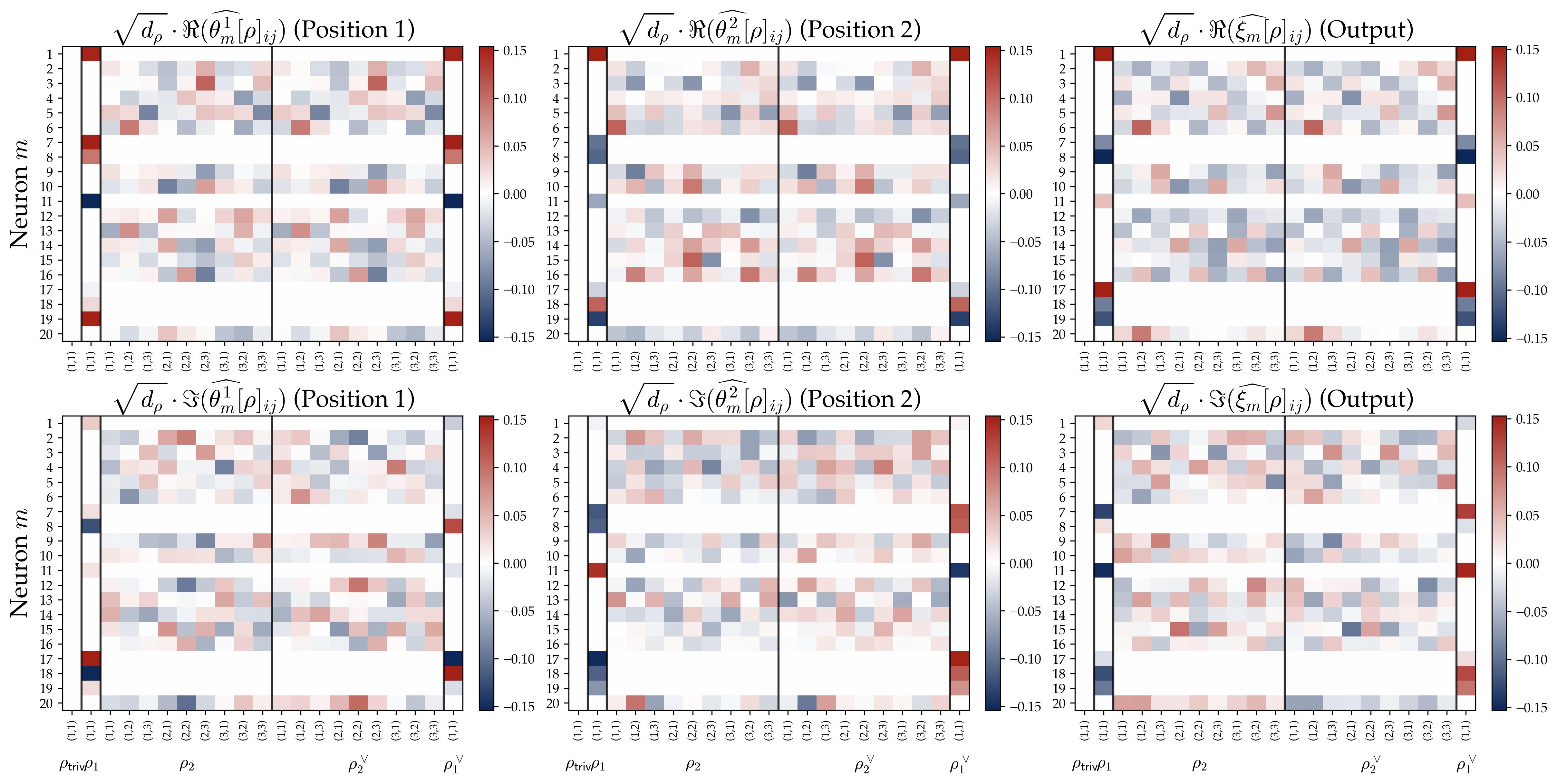
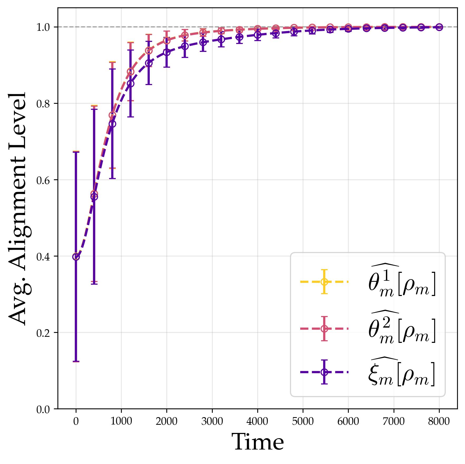
3.5 Experimental Verification: The Frobenius Group $C_7 \rtimes C_3$
We validate the theoretical predictions on the Frobenius group of order 21 described above. Its 3D irreducible representations provide a non-trivial but still manageable arena for observing rank-one alignment.
Experimental setup. We train with $M = 512$ neurons, quadratic activation, and small initialization $a = 0.01$. Stage I runs projected gradient flow for $10^4$ steps; Stage II optimizes scales for $5 \times 10^4$ steps.
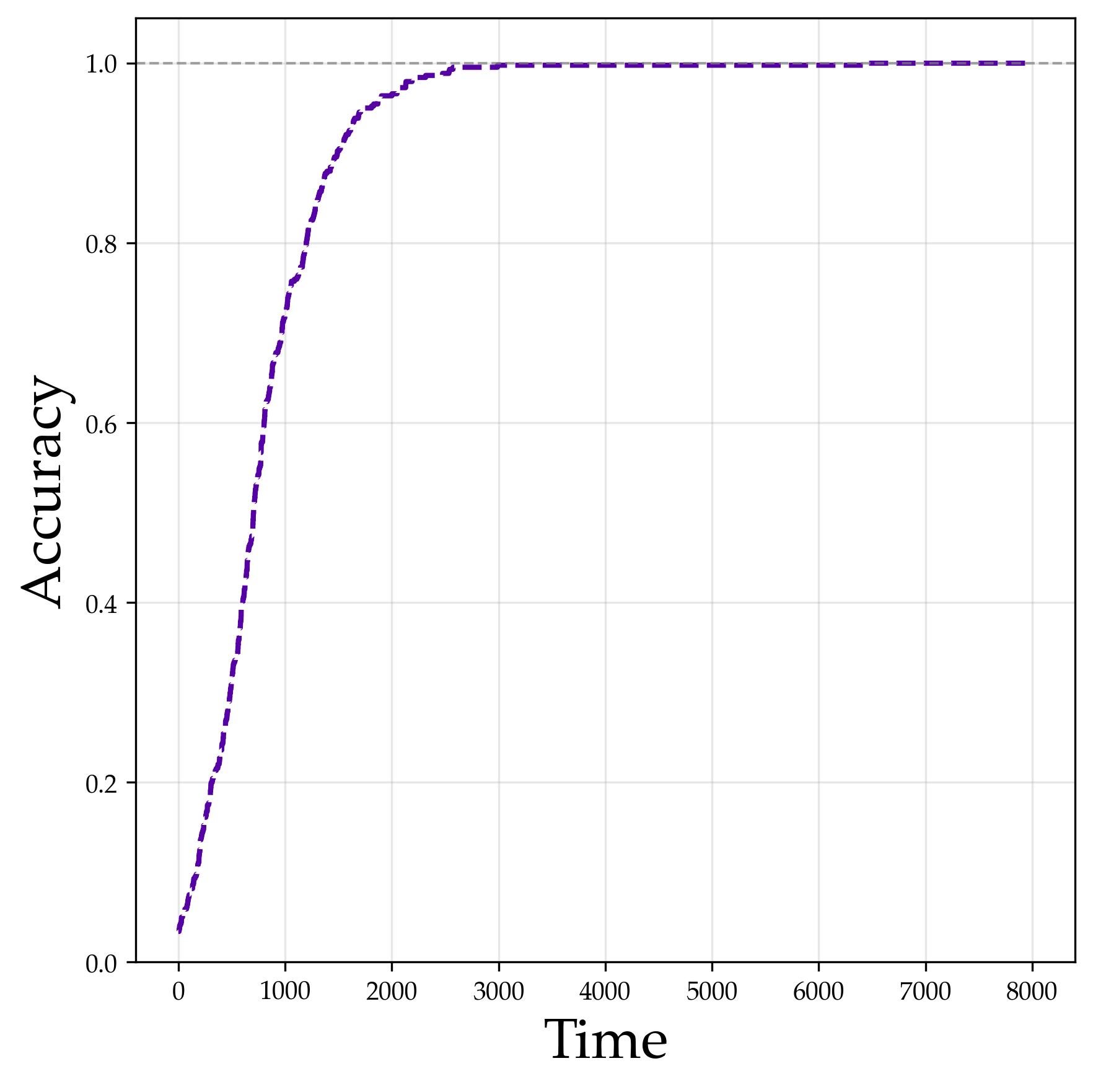
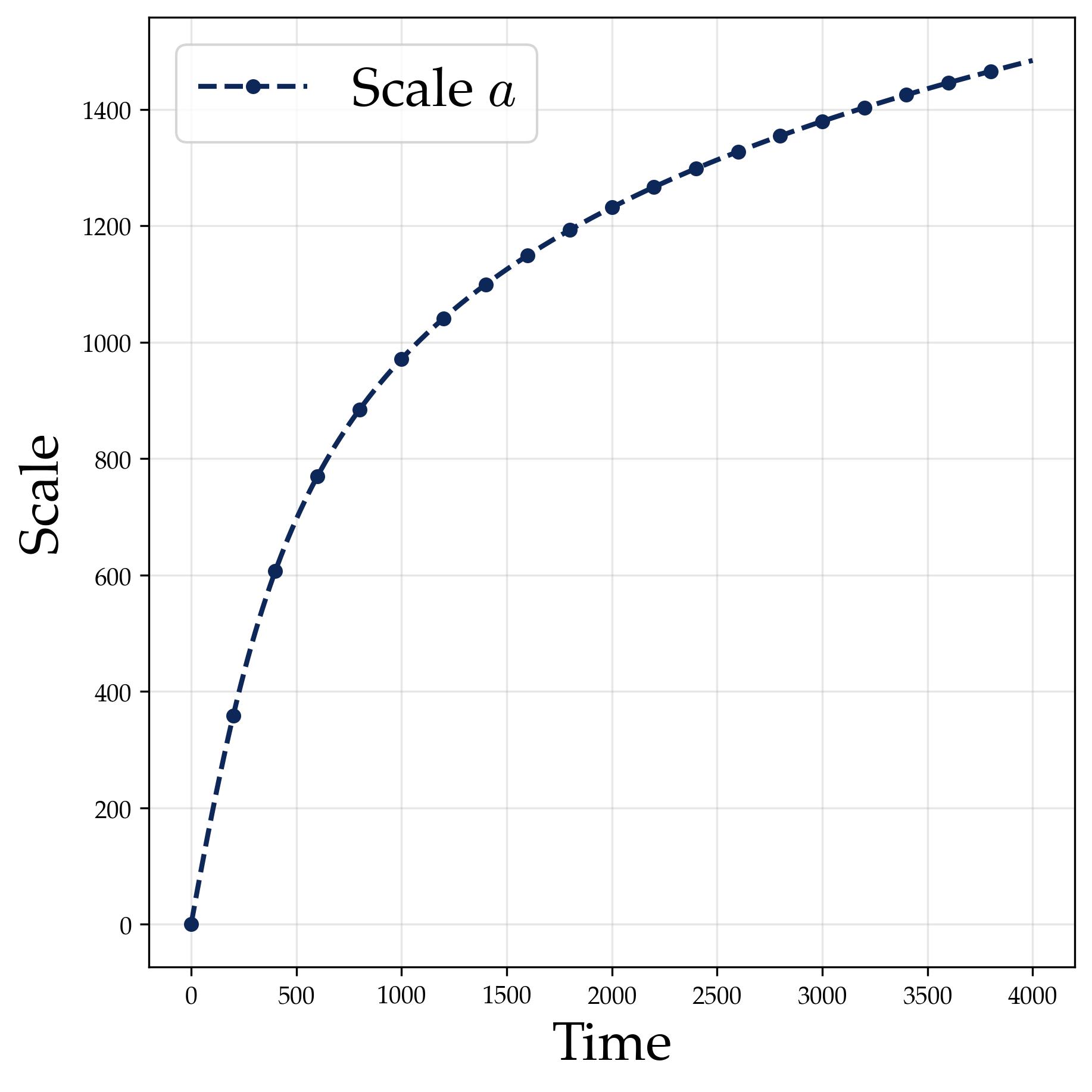
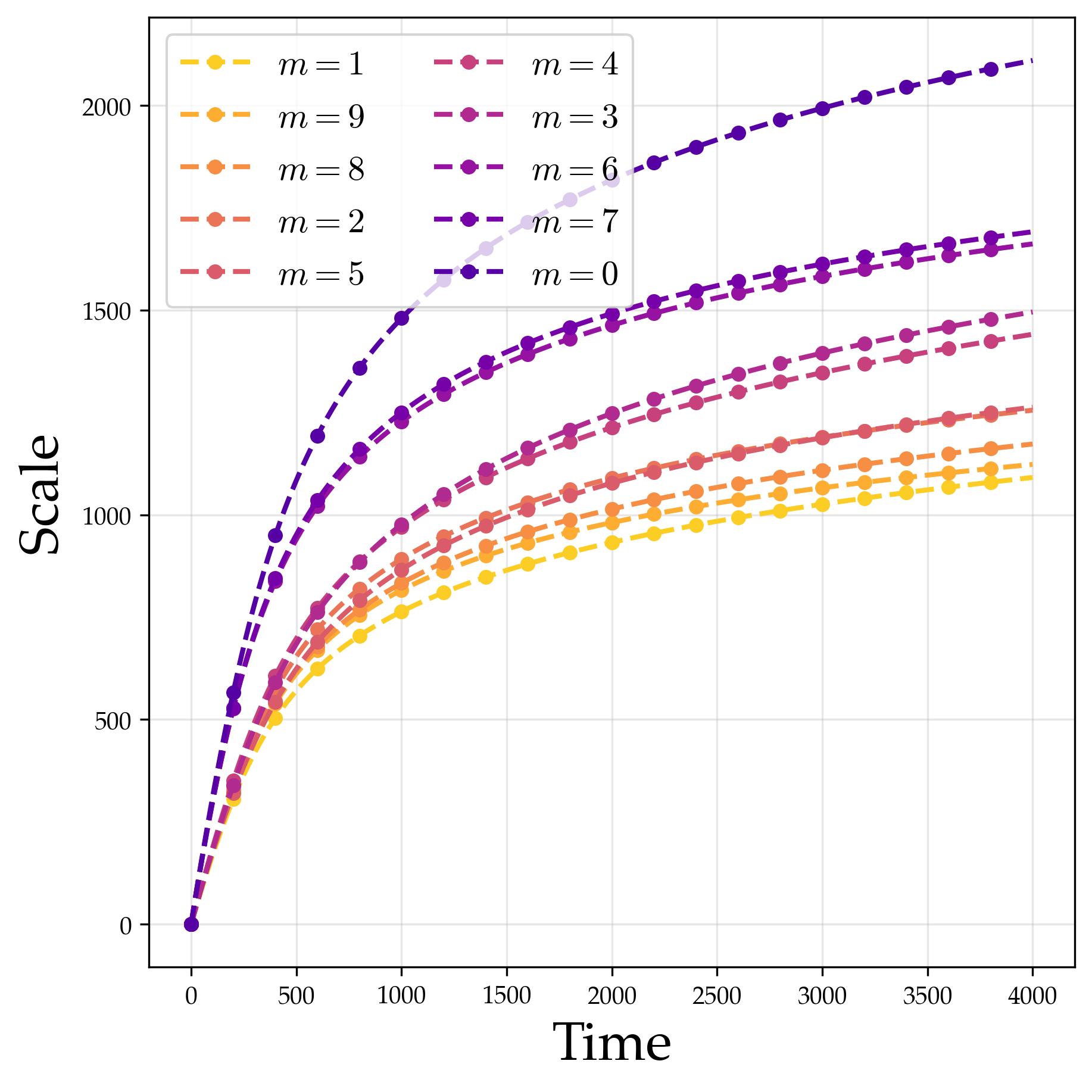
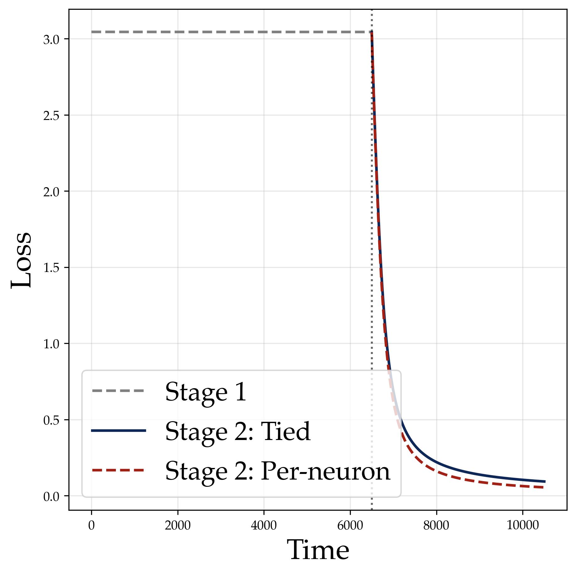
3.6 Stage II: Scale Growth Sharpens Predictions
After Stage I locks in the spectral structure (single representation, rank-one alignment), Stage II grows the scale parameters to reduce the cross-entropy loss. The mechanism is simple: once the logit gap between the correct answer and competitors is established by the directional structure, amplifying all logits by a factor $a$ amplifies the gap proportionally, causing the softmax to concentrate.
Theorem (Stage II Convergence). Suppose the mean-field predictor satisfies the perfect-accuracy condition
$$ \mathcal F_{\sf NN}^{\mu}(g_1,g_2)_{g_1\star g_2}> \max_{j\in G\setminus\{g_1\star g_2\}}\mathcal F_{\sf NN}^{\mu}(g_1,g_2)_j \qquad \forall g_1,g_2\in G. $$If the neuron scales are tied, then for sufficiently wide networks, with high probability,
$$a(t)\gtrsim\log\bigl(1 + |G|(|G|-1)t\bigr),$$and the cross-entropy loss reaches $\epsilon$ once
$$T\gtrsim |G|/\epsilon\cdot\bigl(1+(|G|-1)^{-2}\bigr).$$The condition says that the Stage I predictor already ranks the correct composition $g_1\star g_2$ above every wrong label, before the scale grows. Since $G$ is finite, this strict inequality over all input pairs implies a positive logit margin. Stage II is then a margin-amplification argument: multiplying logits by an increasing scale sharpens a correct argmax into a confident softmax prediction. In the Abelian case, this condition is provable from the refined population analysis above: the flawed-indicator formula gives coefficient $2$ to the correct label and coefficient $1$ to each ghost label, so the correct logit has a strict margin for every input pair. For general non-Abelian groups, the Stage II theorem is stated conditional on this perfect-accuracy margin.
The logarithmic growth $a(t) \sim \log(t)$ is natural: the softmax saturates exponentially in $a$, so the loss gradient $\partial \mathcal{L}/\partial a$ decays as $e^{-\mu a} \sim 1/t$, giving $\dot{a} \sim 1/t$ and hence $a \sim \log t$.
4. Summary
4.1 From Scalars to Matrices: A Hierarchy
The progression from cyclic groups to general groups reveals a clean hierarchy. Spectral sparsity and alignment persist from scalar Fourier modes to matrix-valued irreducible representations; diversification is fully characterized in the Abelian setting and is not part of the general-group theorem.
| Property | Cyclic $\mathbb{Z}_p$ | General Abelian $G_{\mathcal N}$ | General finite $G$ |
|---|---|---|---|
| Spectral sparsity | Single frequency $k$ | Single character $\check\rho$ | Single irrep $\check\rho_m$ and its dual orbit |
| Alignment | Phase: $\psi = 2\phi$ | Phase: $\arg(\hat{\xi}_m[\rho]) = \arg(\hat{\theta}_m^1[\rho]) + \arg(\hat{\theta}_m^2[\rho])$ | Rank-one rotational: $\hat{\xi}_m[\rho] \propto_+ \hat{\theta}_m^2[\rho]\hat{\theta}_m^1[\rho]$ plus cyclic companion relations |
| Rank condition | Automatic ($d_\rho = 1$) | Automatic ($d_\rho = 1$) | Non-trivial: $\mathrm{rank}(\hat{\nu}[\rho]) = 1$ for $\nu\in\{\theta_m^1,\theta_m^2,\xi_m\}$ |
| Diversification | Uniform over frequencies | Uniform over non-trivial characters, with Haar-uniform phases | Not asserted by the general theorem |
The key new phenomenon at the non-Abelian level is rank-one compression. Each irreducible representation $\rho$ provides a $d_\rho^2$-dimensional space of possible Fourier coefficients, yet the network uses only a rank-one slice. The proof mechanism is the Stage I spectral-energy argument described above: stable positive-energy equilibria are exactly the single-irrep, rank-one, rotationally aligned configurations.
Citation
| |